

A Friendly Primer on Geometric Deep Learning
Expertise Level ⭐⭐

Geometric Deep Learning can appear intimidating at first. This article helps ease the learning curve by (1) organizing the topic around its mathematical foundations and (2) introducing it through the unifying concept of symmetry.
Table of Content
Theory
Applications
🛠️ Python Libraries
📚 This Newsletter Articles
Theory
Applications
Manifold & Group-based Learning
Theory
Applications
🛠️ Python Libraries
📚 This Newsletter Articles
Theory
Applications
🛠️ Python Libraries
📚 This Newsletter Articles
Theory
Applications
🛠️ Python Libraries
📚 This Newsletter Articles
🎯 Why this matters
Purpose: Geometric Deep Learning (GDL) empowers data scientists to understand the underlying shape and structure of data. Yet, the topic can feel overwhelming unless approached through the unifying concept of symmetry.
Audience: Data scientists and software engineers eager to learn the basic concepts of geometric deep learning.
Value: Understanding the fundamental role of symmetry in models and non-Euclidean geometry is essential. This article provides an overview of the diverse and higher-order representations of data that emerge from these principles.
⚠️ This article does not present topics such as topology or differential geometry from a rigorous mathematical standpoint - no PhD required!. Rather, the subsequent sections are designed for data scientists and engineers navigating the theoretical foundations of geometric learning without being burdened by mathematical abstractions.
Optional sections with mathematical formulation are specified as 🤖 For math-minded readers
🔁 The Quest for Symmetry
Introduction
The concept of symmetry is central to Geometric Deep Learning.
Symmetry is the organizing principle behind geometric deep learning. It tells you what should not change (invariance) or how things should change (equivariance) when you transform the input [ref 1].
The benefits of symmetry in differential geometry or topology are:
Simplification: Symmetry makes geometry easier to handle by turning intricate geometric problems into simpler algebraic ones.
Insight: It reveals how local and global properties of manifolds are connected, providing a clearer view of their structure.
Applications: In physics, symmetric spaces are central to theories such as general relativity and string theory, which use them to model the universe.
Definitions
The terms symmetry, invariance and equivariance can be confusing.
Symmetry (Webster dictionary): The property of remaining invariant under certain changes (as of orientation in space, of the sign of the electric charge, of parity, or of the direction of time flow) —used of physical phenomena and of equations describing them
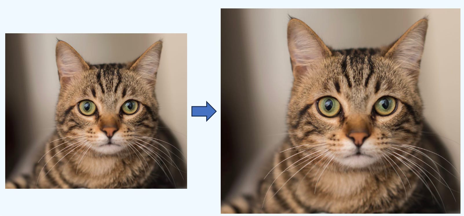
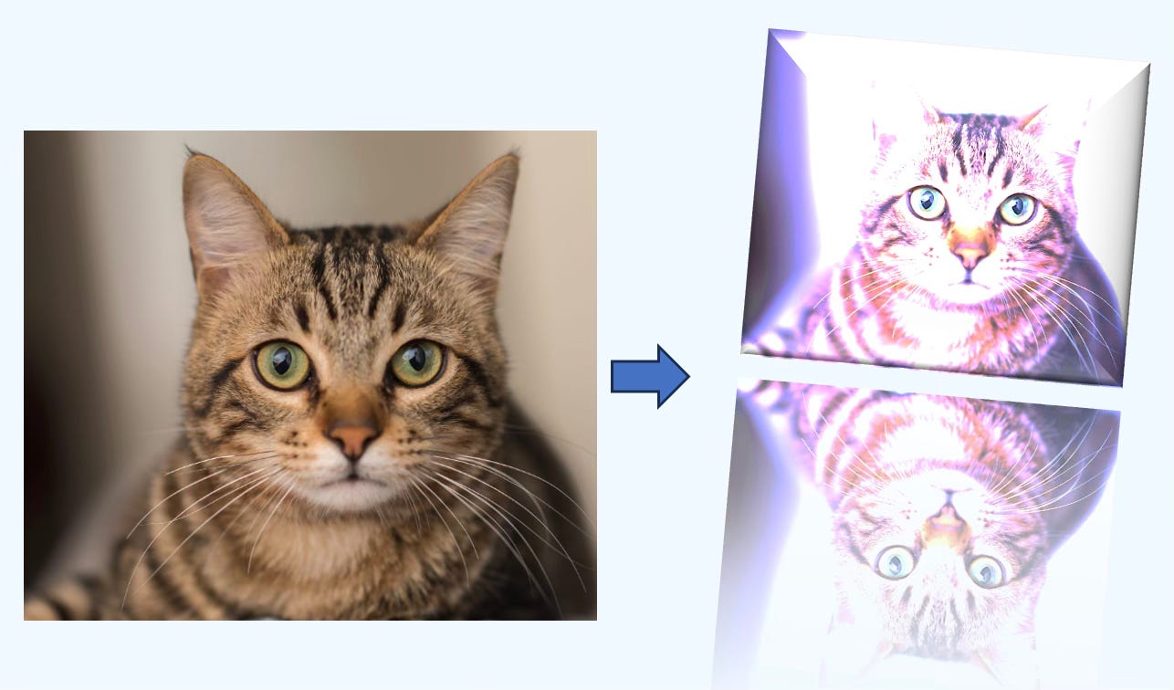
Invariance: The output doesn’t change when the input is transformed. Example: a cat classifier still predicts “cat” for an upside-down photo.
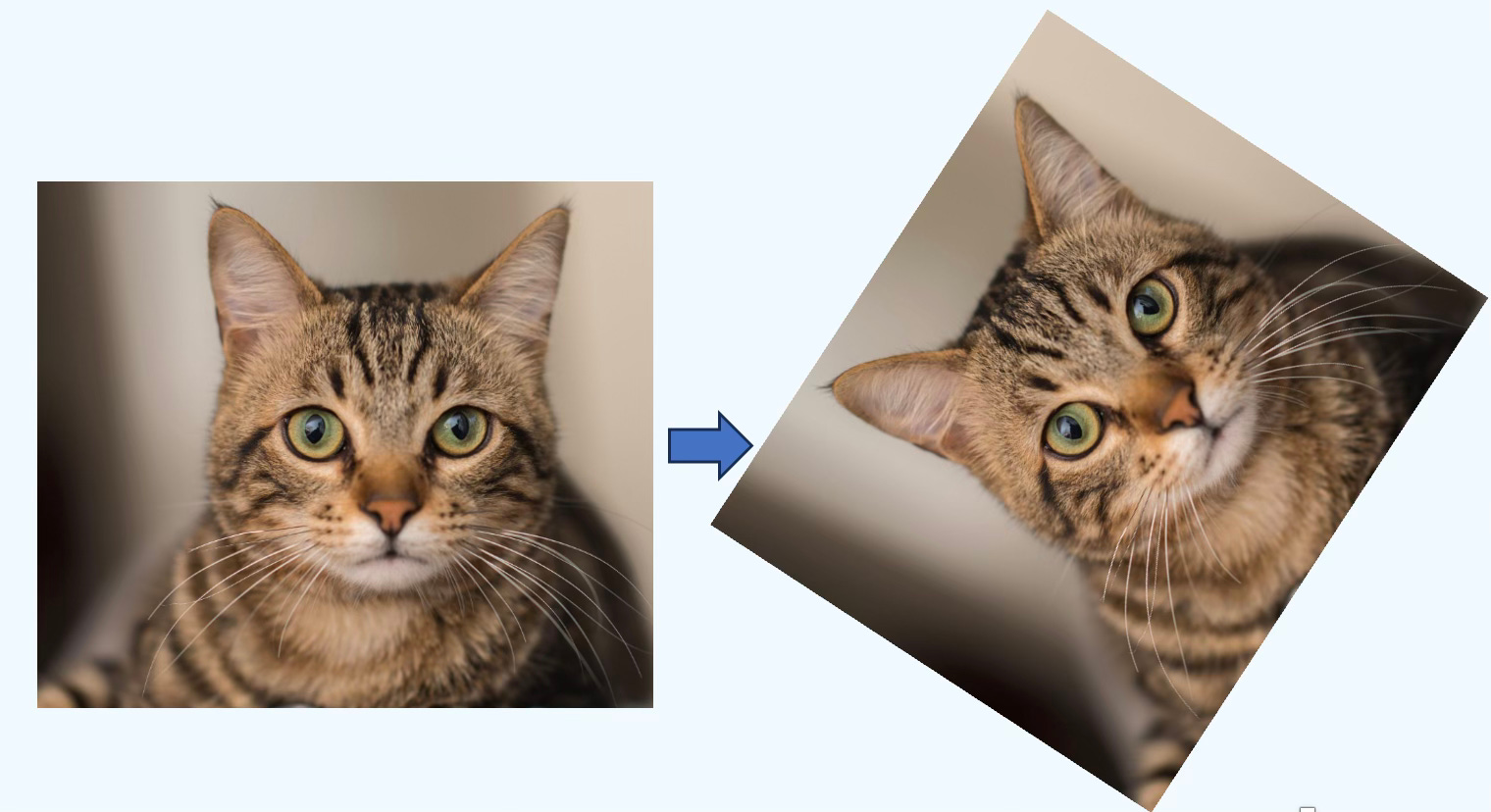
Equivariance: The output changes in a predictable way under the same transformation. Example: rotate an image, and the predicted segmentation mask rotates accordingly.
🤖 For math-minded readers
A function f is invariant, given a group G if for any transformation g
A function f is equivariant, given a group G if for any transformation g, a group action on input rho|x and a group action on outputs rho|y
The relation is simplified in the case the group actions are identical
Finally, the simple scenario of no group actions.
📌 The formulation of invariance and equivariance varies depends on the field they apply such as Metric, Laplace-Beltrami operator, Lie derivative orTensor field.
Symmetry in Images
The concept of symmetry and invariance can be easily illustrated in the context of computer vision. Vision models are often trained to be invariant to common geometric transforms:
Translation: horizontal/vertical shifts; the object is recognized regardless of image location.

Rotation: turning the image by some angle.
Scaling: resizing the object.
Affine transforms: compositions of translation, rotation, scaling, and shear; they preserve straightness and parallel lines.

Projective transforms: changes in camera viewpoint; lines remain straight but parallels may meet at a vanishing point, which is especially challenging.
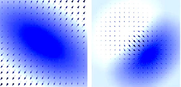
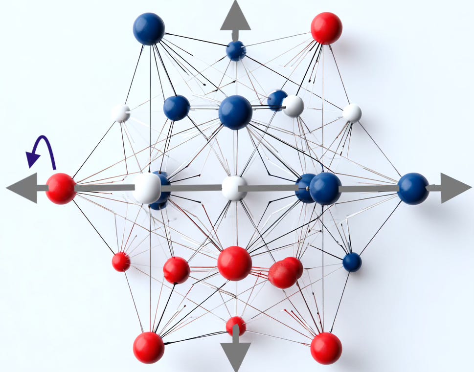
Symmetry in Shapes
Symmetric shapes arise in many applications and scientific domains.
Differential geometry & manifold learning: the gradient and divergence operators on vector fields often exhibit symmetric patterns.
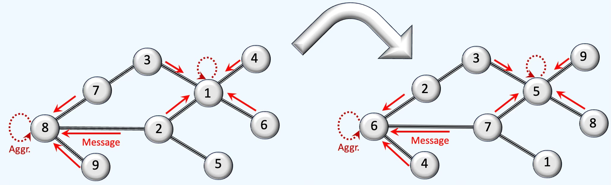
Graphs: repeating motifs appear in colored, undirected graphs.
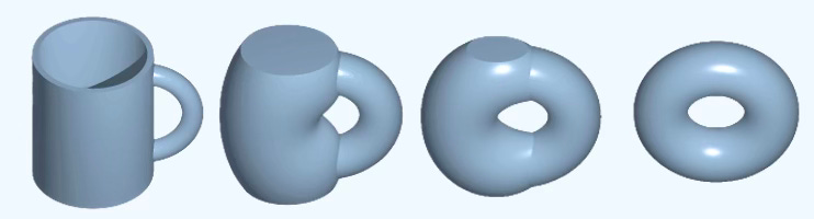
Homotopy (algebraic topology): studies continuous deformations of shapes and relates closely to equivariance.
Graph Neural Networks: exploit permutation invariance of node indices.
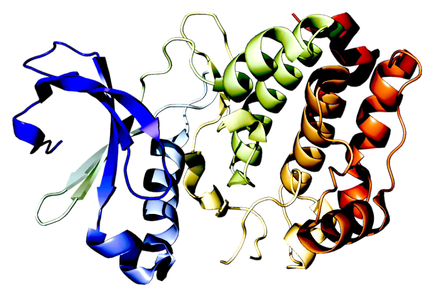
Biochemistry: components of Aurora A kinase (a serine/threonine kinase) inhibitors for tumor-suppressor pathways show notable structural similarities.
Symmetry in Mathematics
Beyond geometry, symmetric (and sometimes antisymmetric) patterns appear throughout mathematics. Here are some examples:
Convolution (in the usual linear/abelian setting) is commutative
The Lie bracket is the algebraic operation that captures how infinitesimal symmetries interact. The symmetry is abelian if the bracket is null.
The special orthogonal group SO(3)—the rotations of 3-dimension Euclidean space—is a continuous symmetry (Lie) group acting on space.
The tensor product of vector spaces comes with a universal bilinear map with symmetry property.
The wedge product is antisymmetric and equivariant under linear transformations T. It is invariant under rotations
📌 A final note: Symmetry play an important role in World Models where reasoning task such as prediction, planning or simulation are performed entirely in the latent space.
🧮 Geometric Deep Learning
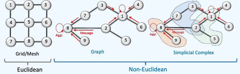
Geometric Deep Learning (GDL) is a branch of machine learning dedicated to extending deep learning techniques to non-Euclidean data structures. Currently, there is no universally agreed-upon, well defined scope for Geometric Deep Learning, as its interpretation varies among authors.
GDL unlocks the ability to model complex, structured, and relational data, enabling advanced problem-solving in areas like social networks, molecular science, design optimization, and transportation systems.
Geometric Deep Learning (GDL) has been introduced by M. Bronstein, J. Bruna, Y. LeCun, A. Szlam and P. Vandergheynst in 2017 [ref 2]. Readers can explore the topic further through a tutorial by M. Bronstein [ref 3, 4].
⚠️ This article does not delve into the mathematical foundations of Geometric Deep Learning—such as topology or differential geometry—which were covered in a previous article [ref 5] and comprehensively detailed in the excellent paper Mathematical Foundations of Geometric Deep Learning [ref 6].
We arbitrary break down the field into 5 categories
Graph Neural Networks
Mesh Modeling
Manifold & Group-Based Learning
Topological Deep Learning
Information-Geometric Learning
📌 The layout of this article traces the evolution of geometry in learning systems—from discrete structures to discretized continuums, onward to continuous and differential, then global, and finally statistical geometry. Within this continuum, meshes act as the intermediary stage, rooted in discrete differential geometry and linking Graph Neural Networks to manifold learning.
Graph Neural Networks
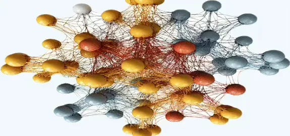
A Graph Neural Network (GNN) is an optimizable transformation on all attributes of the graph (nodes, edges, global context) that preserves graph symmetries (permutation invariances). GNN takes a graph as input and generate/predict a graph as output [ref 7, 8].
Theory
Data on manifolds can often be represented as a graph, where the manifold’s local structure is approximated by connections between nearby points. Graph Neural Networks (GNN) and their variants (like Graph Convolutional Networks (GCNs)) extend neural networks to process data on non-Euclidean domains by leveraging the graph structure, which may approximate the underlying manifold [ref 9, 10, 11].
💡 Inductive vs Transductive Modes
Inductive GNNs learn from existing (training) and new, unseen nodes, links or graphs (inference). There is no need for these models to store and node/link embeddings [ref 12].
Transductive graph models are trained on the complete, fully defined graph (all nodes and edges). As a result, they tend to overfit the training set and struggle to generalize to unseen nodes, edges, or entirely new graphs. Their message passing and aggregation schemes are typically straightforward.
💡 Graph Metrics
The selection of the topology of a GNN depends on centrality and homophily among other metrics.
The various centrality measures quantify a node’s (or edge’s) structural importance so you can prioritize, rank, or act on parts of the network.
🔹 Degree Centrality – Who’s most connected?
🔹 Closeness Centrality – Who’s closest to everyone?
🔹 Betweenness Centrality – Who bridges others?
🔹 Eigenvector Centrality – Who’s connected to the important ones?
🔹 PageRank – Who’s most influential?
🔹 Clustering Coefficient – Who’s in tight-knit groups?
🔹 Graph Density – How connected is the network?
🔹 Connected Components – How many isolated groups exist?
Homophily provides a principled way to assess whether proximity in the graph structure—through nodes or edges—correlates with similarity in labels or classes [ref 13]. In a nutshell, Edge homophily answers: “How likely is it that a random edge connects same-label nodes?” while Node homophily answers: “How homophilic is the neighborhood of a typical node?.
🤖 For math-minded readers
Let’s start with the mathematical definition. Let G=(V,E) be a graph with a set of nodes (vertices) V, a set of edges E, label yv of node v and a neighbors of node v, N(v), there are 3 types of homophily ratios:
Node homophily ratio: Average fraction of same-label neighbors per node.
Edge homophily ratio: The fraction of edges in a graph which connects nodes that have the same class label.
Class insensitive edge homophily ratio: Edge homophily is modified to be insensitive to the number of classes and size of each class. C number of classes, |Ck| number of nodes of class k and hk denotes the edge homophily ratio of class k.
💡 Common types
Detailed information is available in a previous article [ref 14].
Graph Convolutional Networks (GCNs): GCNs generalize the concept of convolution from grids (e.g., images) to graphs. They aggregate information from a node’s neighbors using normalized adjacency matrices and apply transformations to learn node embeddings.
Spectral Graph Neural Networks (SGNN): These networks operate in the spectral domain using the graph Laplacian. They use eigenvectors of the Laplacian for convolution-like operations.
Relational Graph Convolutional Networks (R-GCNs):R-GCNs extend GCNs to handle heterogeneous graphs with different types of nodes and edges.
Graph Transformers: They adapt the Transformer architecture to graph-structured data using attention mechanisms and global context.
Graph Autoencoders: These are used for unsupervised learning on graphs, aiming to reconstruct graph structure and node features.
Diffusion-Based GNNs: These networks use graph diffusion processes to propagate information. The vast majority of research papers train these models in transductive mode although it can theoretically be run in inductive mode.
GraphSAGE (Graph Sample and Aggregate) learns node embeddings by sampling and aggregating features from a fixed-size neighborhood of each node, enabling scalable learning on large graphs.
Graph Attention Networks (GATs) use attention mechanisms to learn the importance of neighboring nodes dynamically. Each edge is assigned a learned weight during aggregation that doesn’t depend on the specific training graph’s Laplacian.
Graph Isomorphism Networks (GINs): GINs are designed to be as powerful as the Weisfeiler-Lehman (WL) graph isomorphism test, distinguishing graph structures more effectively.
Graph Pooling Networks: They summarize graph information into a smaller representation, similar to pooling in CNNs. They can be categorized into Global and hierarchical pooling. Spectral pooling methods that depend on a graph’s specific eigenbasis are generally transductive to that graph.
Hyperbolic Graph Neural Networks: These networks operate in hyperbolic space, which is well-suited for representing hierarchical or tree-like graph structures).
Dynamic Graph Neural Networks: These networks are designed to handle temporal graphs, where nodes and edges evolve over time.
Applications
Graph classification
Molecules: property prediction, docking, affinity, generative design, retro-synthesis.
Biology: structure graphs for residue, Protein-Protein interaction function prediction, fold & complex modeling.
Chemistry: force fields, Δ-learning for Discrete Fourier Transform, reaction outcome prediction.
Vision: point clouds & meshes, scene classification, segmentation, pose.
Software Engineering: bug detection, optimization, code similarity.
Routing: placement & layout optimization.
Finance: default risk, alpha signals.
…
Node classification & Link prediction
Recommenders: user–item graphs; link prediction for Click Through Ratio, cold-start, ranking.
Risk Analysis: transaction networks, identity graphs; anomaly detection, entity resolution.
Cybersecurity: log graphs, call graphs; suspicious edge & node detection.
Knowledge Graphs: entity/relation reasoning
Healthcare: patient–event graphs for Electronic Health Records, disease–gene networks & risk prediction.
…
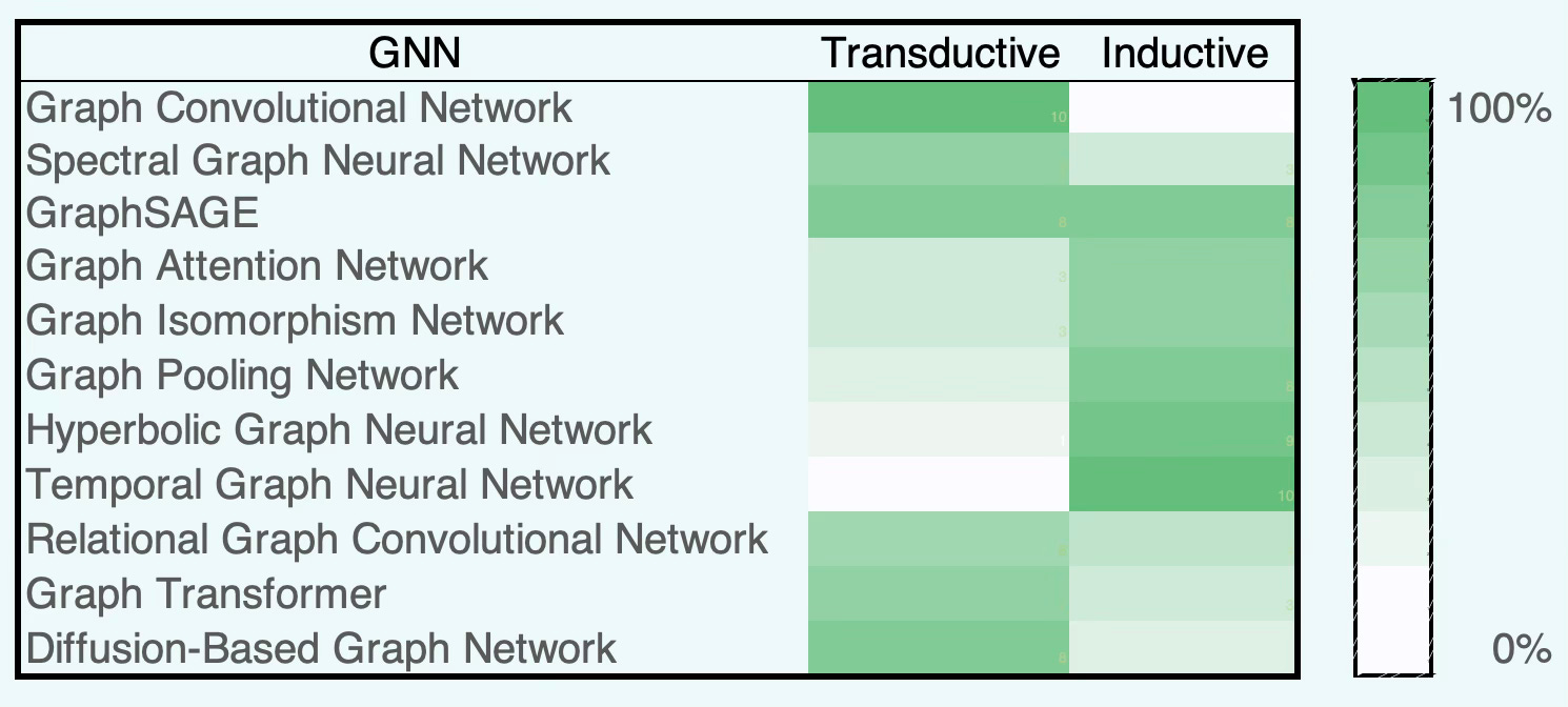
⚠️ As seen in this section, the distinction between transduction and induction is a bit fuzzy. For instance a Graph Isomorphism Network) applies to unseen graph and therefore is inductive. However it can be run transductively on a single fixed graph for node classification.
The table below categorizes the most common Graph Neural Networks according to their training paradigm—transductive, inductive, or a combination of both. The intensity of the green shading indicates approximately the relative proportion between transductive and inductive modes.
📌 The principles of graph theory serve as the mathematical backbone of Graph Neural Networks, guiding their configuration and performance optimization [ref 15, 16, 17, 18 & 19].
🛠️ Python Libraries
PyTorch Geometric
PyTorch Geometric (PyG) has emerged as a leading library for exploring and implementing GNNs using PyTorch [ref 20]. However, the vast array of available models and techniques can be overwhelming.
Its key features of PyTorch Geometric are:
Efficient Graph Processing: Optimizes memory and computation using sparse graph representations.
Flexible GNN Layers: Covers GCN, GAT, GraphSAGE, GIN, and other advanced architectures.
Batching for Large Graphs: Supports for mini-batching for handling graphs with millions of edges.
Seamless PyTorch Integration: Provides full compatibility with PyTorch tensors, autograd, and neural network modules.
Diverse Graph Support: PyTorch Geometric handles directed, undirected, weighted, and heterogeneous graphs.
pip install torch_geometricNetworkX
NetworkX is a BSD-license powerful and flexible Python library for the creation, manipulation, and analysis of complex networks and graphs. It supports various types of graphs, including undirected, directed, and multi-graphs, allowing users to model relationships and structures efficiently.
NetworkX provides a wide range of algorithms for graph theory and network analysis, such as shortest paths, clustering, centrality measures, and more. It is designed to handle graphs with millions of nodes and edges, making it suitable for applications in social networks, biology, transportation systems, and other domains. With its intuitive API and rich visualization capabilities, NetworkX is an essential tool for researchers and developers working with network data.
The library supports many standard graph algorithms such as clustering, link analysis, minimum spanning tree, shortest path, cliques, coloring, cuts, Erdos-Renyi or graph polynomial.
Installation
pip install networkx📌 These libraries have been described in details in a previous article Taming PyTorch Geometric for Graph Neural Networks [ref 22].
📚 This Newsletter Articles
Neighbors Matter: How Homophily Shapes Graph Neural Networks
Demystifying the Math of Geometric Deep Learning - Graph Theory
Introduction to Geometric Deep Learning - Graph Neural Networks
Mesh Modeling
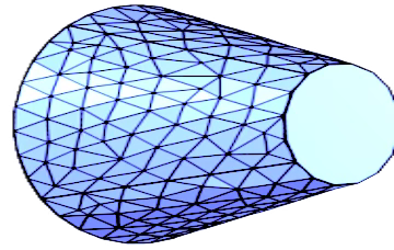
A mesh in discrete differential geometry is a finite, piecewise-linear approximation of a smooth geometric object. The most common type are simplicial and combinatorial complexes (vertices, edges, faces) together with a geometric embedding of its vertices in Rn (most often 3D). The mesh supplies the discrete scaffold on which smooth notions—metric, curvature, differential operators—are defined and computed.
Theory
While a Riemannian manifold in differential geometry models data in a continuous domain, a mesh—rooted in discrete differential geometry [ref 23]—represents data through a structured assembly of interconnected topological elements.
Point clouds consist of discrete 3D points—typically captured by 3D scanners or depth cameras—where each point is defined by its spatial coordinates (X, Y, Z) and may carry extra attributes such as color or intensity. They offer a flexible way to represent the geometry of real-world objects or scenes without requiring explicit connectivity between points.
Meshes, in contrast, are structured collections of vertices, edges, and faces that together define the surface of a 3D object. Unlike point clouds, they encode explicit topological relationships between elements, providing a continuous surface representation. Meshes are widely used in 3D modeling, computer graphics, and additive manufacturing (3D printing).
A mesh is the discrete surface/volume on which we do geometry: it carries both the topology (connectivity) and the metric (lengths/areas/angles), enabling faithful, stable discretization of smooth geometric operators.
A triangle mesh is a manifold, but only if
Every edge is incident to exactly 2 faces or 1 face
Every triangle incident to each of its vertices is homeomorphic to a disk or half-disk.
Meshes are related to persistent homology.
The cotangent Laplacian is the standard discrete Laplace–Beltrami operator on a triangle mesh. It’s the matrix you get when you discretize the continuous Laplacian using piecewise-linear (P1) finite elements; its edge weights are built from triangle cotangents. The cotangent Laplacian is derived from the Dirichlet energy.
Applications
3D shape classification & retrieval: Mesh CNNs or spectral GNNs process vertices and faces with DDG-derived operators.
Surface reconstruction: Deep neural-mesh methods rebuild smooth surfaces from point clouds.
Differentiable simulation: Learn physical parameters (e.g., Young’s modulus) using mesh-based finite element method.
Physics-informed neural networks on meshes: Uses unstructured meshes instead regular (Euclidean) grids.
Surface-based graph learning: Message passing over vertex adjacency with geometric weights from discrete differential geometry.
Surface smoothness loss: Regularize geometry by penalizing curvature variation
3D reconstruction in computer vision: Mesh prediction networks for deformable surfaces.
Articulated object modeling: Jointed mesh deformations (e.g., human body models)
Scene understanding: Meshes integrated with point clouds for semantic segmentation and navigation.
…
Manifold & Group-Based Learning
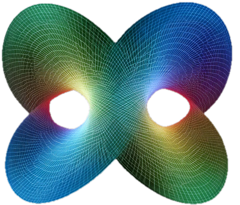
Machine learning models based on manifolds leverage differential geometry [ref 24]. A manifold is essentially a space that, around every point, looks like Euclidean space, created from a collection of maps (or charts) called an atlas, which belongs to Euclidean space.
Theory
Differential (or smooth) manifolds have a tangent space at each point, consisting of vectors. Riemannian manifolds are a type of differential manifold equipped with a metric to measure curvature, gradient, and divergence
The primary goal of learning Riemannian geometry is to understand and analyze the properties of curved spaces that cannot be described adequately using Euclidean geometry alone.
💡 Differential Geometry
Differential geometry is an extensive and intricate area that exceeds what can be covered in a single article or blog post. There are numerous outstanding publications, including books [ref 25, 26 & 27], this newsletter article [ref 28] and tutorials [ref 29, 30], that provide foundational knowledge in differential geometry and tensor calculus, catering to both beginners and experts
💡 Smooth Manifolds
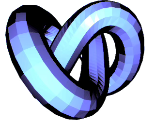
A manifold is a topological space that, around any given point, closely resembles Euclidean space. Specifically, an n-dimensional manifold is a topological space where each point is part of a neighborhood that is homeomorphic to an open subset of n-dimensional Euclidean space. Examples of manifolds include one-dimensional circles, two-dimensional planes and spheres, and the four-dimensional space-time used in general relativity.
Smooth or Differential manifolds are types of manifolds with a local differential structure, allowing for definitions of vector fields or tensors that create a global differential tangent space.
A Riemannian manifold is a differential manifold that comes with a metric tensor, providing a way to measure distances and angles [ref 31].
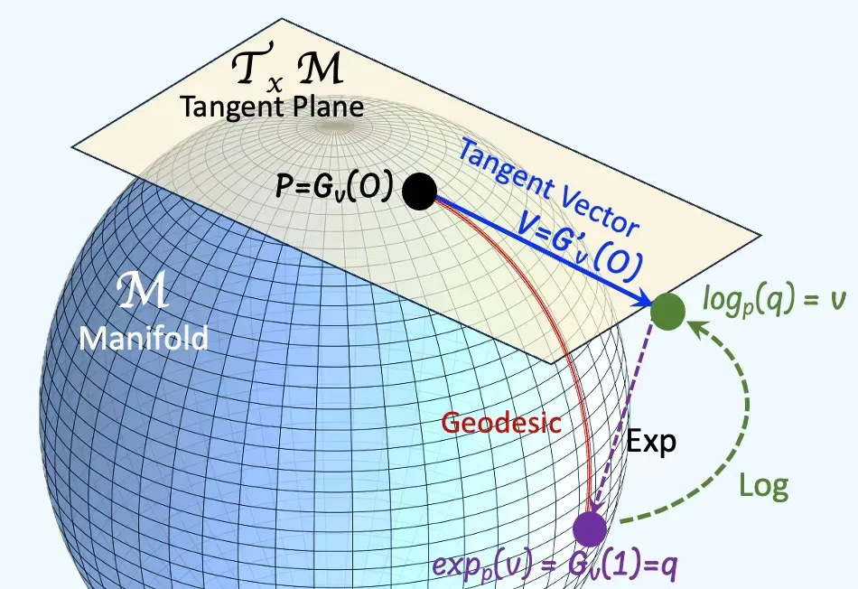
The tangent space at a point on a manifold is the set of tangent vectors at that point, like a line tangent to a circle or a plane tangent to a surface. Tangent vectors can act as directional derivatives, where you can apply specific formulas to characterize these derivatives.
Intuitively, the directional derivative measures how a function changes as you move in a specific direction. The directional derivative
is large and positive, the function is increasing quickly in that direction.
is zero, the function doesn’t change in that direction.
is negative, the function is decreasing in that direction.
💡 Riemannian Geometry
A geodesic is the shortest path between two points on a surface, volume or high dimension space it lives in. It is a straight line on a plane, a curve on a sphere similar to the trajectory of a airplane on a long-haul route.
The exponential map translates an initial direction and velocity—represented by a tangent vector at a given point—into a new point on the manifold reached by following the geodesic that starts in that direction for a unit amount of time. Conceptually, it provides a way to move from the linear world (tangent space) to the curved world (manifold) while preserving the notion of “straight motion.”
The logarithm map does the inverse: it takes two points on the manifold and expresses the shortest displacement between them as a tangent vector in the tangent space of one of the points.
In essence, it “flattens” the manifold locally so that the difference between two points can be represented linearly. This operation enables linear reasoning, differentiation, and optimization on curved domains—allowing algorithms to work with familiar linear tools in the tangent space and then project results back onto the manifold via the exponential map.
The exponential and logarithm maps form a conceptual bridge between local linear geometry and global curved geometry. They are essential in Riemannian optimization, geometric statistics, and manifold-based machine learning because they enable movement, interpolation, and computation on non-Euclidean spaces using local linear approximations while respecting the manifold’s curvature and structure.
🤖 For math-minded readers
Given a Riemannian manifold M with a metric tensor g, the geodesic length L of a continuously differentiable curve f: [a, b] -> M
An exponential map is a map from a subset of a tangent space of a Riemannian manifold. Given a tangent vector v at a point p on a manifold, there is a unique geodesic Gv and an exponential map exp.
Given a differentiable function f, a vector v in Euclidean space Rn and a point x on manifold, the directional derivative in v direction at x is defined as:
A Riemannian metric on a smooth manifold M is a choice, at every point of M, of an inner product on the tangent space that varies smoothly with the point. Formally, it’s a smooth, symmetric, positive-definite (0,2)-tensor field [ref 32].
Parallel transport moves a vector along a curve on a manifold so that it stays “as unchanged as possible” according to the manifold’s connection.
The Levi–Civita connection is the canonical way to differentiate vector fields on a Riemannian manifold that satisfies two conditions - Torsion free & metric compatibility [ref 33].
Riemannian curvature measures how a Riemannian manifold bends—i.e., how its geometry deviates from flat Euclidean space. Tt encodes how a vector changes after parallel transport around a tiny loop (holonomy). On a Riemannian manifold with Levi–Civita connection, a vector field along a smooth curve is parallel if its covariance derivative is null.
Ricci curvature is a way to estimate the full Riemann curvature tensor by averaging sectional curvatures through each tangent direction.
Ricci flow is a geometric evolution equation that smooths a Riemannian metric by diffusing its curvature. It can be interpreted as the heat equation for the metric: regions of high curvature diffuse out, tending to uniformize the geometry [ref 34].
Intrinsic geometry involves studying objects, such as vectors, based on coordinates (or base vectors) intrinsic to the manifold’s point. For example, analyzing a two-dimensional vector on a three-dimensional sphere using the sphere’s own coordinates
Extrinsic geometry in differential geometry deals with the properties of a geometric object that depend on its specific positioning and orientation in a higher-dimensional space.
Here’s what extrinsic geometry involves:
Embedding: Extrinsic geometry examines how a lower-dimensional object, like a surface or curve, is situated within a higher-dimensional space.
Extrinsic coordinates: These are coordinates that describe the position of points on the geometric object in the context of the larger space.
Normal vectors: An important concept in extrinsic geometry is the normal vector, which is perpendicular to the surface at a given point. These vectors help in defining and analyzing the object’s orientation and curvature relative to the surrounding space.
Curvature: Extrinsic curvature measures how a surface bends within the larger space.
Projection and shadow: Extrinsic geometry also looks at how the object projects onto other surfaces or how its shadow appears in the ambient space.
🤖 For math-minded readers
The Riemann metric g is defined as
Christoffel symbol for a Levi-Civita Connection equipped with a Riemannian metric g
Riemann curvature tensor using Christoffel symbols
Ricci curvature as contraction of the Riemann curvature tensor
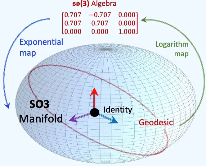
💡 Lie Groups & Algebras
Lie groups play a crucial role in Geometric Deep Learning by modeling symmetries such as rotation, translation, and scaling. This enables non-linear models to generalize effectively for tasks like object detection and transformations in generative models [ref 35, 36 & 37]
In differential geometry, a Lie group is a mathematical structure that combines the properties of both a group and a smooth manifold. It allows for the application of both algebraic and geometric techniques. As a group, it has an operation (like multiplication) that satisfies 4 axioms:
Closure
Associativity
Identity
Invertibility
A Lie algebra is a mathematical structure that describes the infinitesimal symmetries of continuous transformation groups, such as Lie groups. It consists of a vector space equipped with a special operation called the Lie bracket, which encodes the algebraic structure of small transformations. Intuitively, a Lie algebra is a tangent space of a Lie group.
The Special Euclidean Group [ref 38] and Special Orthogonal Group [ref 39] are the most commonly applied Lie groups.
🤖 For math-minded readers
— Special Orthogonal Groups SO(2), SO(3)
The Special Orthogonal Groups SO(2) (resp. SO(3)) are the Lie groups that represents rotations in 2-dimensional (resp. 3-dimensional) space. It is widely used in robotics, physics, computer vision, and geometric deep learning to describe rigid body rotations without scaling or reflection.
— Special Euclidean Group SE(3)
The Special Euclidean group is a subset of the broader affine transformation group. It contains the translational and orthogonal groups as subgroup. In robotics and physics, an element of SE(3) is often referred to as a rigid transformation, since it describes a rotation + translation without scaling or deformation.
Applications
The following highlights the advantages of utilizing differential geometry to tackle the difficulties encountered by researchers in the creation and validation of generative models.
Understanding data manifolds: Data in high-dimensional spaces often lie on lower-dimensional manifolds.
Improving latent space interpolation: In generative models, navigating the latent space smoothly is crucial for generating realistic samples. .
Optimization on manifolds: The optimization processes used in training generative models can be enhanced by applying differential geometric concepts.
Geometric regularization: Incorporating geometric priors or constraints based on differential geometry can help in regularizing the model.
Advanced sampling techniques: Differential geometry provides sophisticated techniques for sampling from complex distributions (important for both training and generating new data points).
Enhanced model interpretability: By leveraging the geometric structure of the data and model, differential geometry can offer new insights into how generative models work.
Physics-Informed Neural Networks: Projecting physics law and boundary conditions such as set of partial differential equations on a surface manifold improves the optimization of deep learning models.
3D rotations & poses: SO(3), SE(3) manifolds for robotics, molecular dynamics, pose estimation.
Shape analysis: manifold of diffeomorphisms or curves for medical imaging and object alignment.
Computer vision: intrinsic geometry of images, geodesic flows between shapes.
Differential equations: Neural ODEs and continuous normalizing flows on manifolds.
Graph: Node embedding on manifolds
Word embeddings: Poincare (hyperbolic) embeddings
Simulation: Heat-flow using Laplace-Beltrami operator
Clustering & regression: Information geometry and geodesic distances
Bain-connectivity, MRI & EEG: Symmetric Positive Definite (SPD) groups
Low-rank factorization, PCA: Stiefel & Grassmann manifolds
Robotics: Special orthogonal groups and Special Euclidean groups in 3 dimension
Taxonomy & knowledge graphs: Hyperbolic manifolds
Encoding directional data: Spherical manifolds
…
🛠️ Python Libraries
Geomstats
The core concept of Geomstats is to incorporate differential geometry principles, such as manifolds and Lie groups, into the development of statistical and machine learning models [ref 40]. This open-source, object-oriented library follows Scikit-Learn’s API conventions for seamless integration.
Geomstats serves as a practical tool for gaining hands-on experience with geometric learning fundamentals while also supporting future research in the field [ref 41].
This article focuses on the following 3 Geomstats modules:
geometry
information geometry
learning
Installation (Linux/Mac)
pip install geomstatsPymanopt
Pymanopt is a modular and user-friendly toolbox that abstracts away the complexity of Riemannian optimization [ref 42]. Automatic differentiation is handled transparently, minimizing the setup required from the user. It relies on NumPy and SciPy, and supports built-in automatic differentiation through cost functions defined in Autograd (JAX), TensorFlow, or PyTorch.
Installation (Linux/Mac)
pip install “pymanopt[autograd]” 📌 Geomstats has been described in details in a previous article Exploring Geometric Learning with Geomstats [ref 43].
📚 This Newsletter Articles
Demystifying the Math of Geometric Deep Learning - Differential Geometry
Introduction to Geometric Deep Learning - Data Manifolds & Groups
Topological Deep Learning
Topological Deep Learning (TDL) is an emerging area of machine learning that extends traditional deep learning and graph neural networks (GNNs) to operate on higher-order topological structures beyond simple graphs [ref 44, 45]. While GNNs model pairwise relationships (nodes and edges), TDL leverages the mathematics of algebraic topology to capture multi-way interactions (e.g., triangles, tetrahedra) and topological invariants like holes, cycles, and cavities [ref 46].

Theory
💡 Point Set Topology
Point-set (general) topology treats the foundational definitions and constructions of topology. Key concepts include continuity (pre-images of open sets are open), compactness (every open cover admits a finite sub-cover), and connectedness (no separation into two disjoint nonempty open subsets) [ref 47].
A topological space is a set equipped with a topology—a collection of open sets (or neighborhood system) satisfying axioms that capture “closeness” without distances. It may or may not arise from a metric. Common examples include Euclidean spaces, metric spaces, and manifolds.
💡 Category Theory
Category theory offers a panoramic view of mathematics: it suppresses detail to reveal structure. From this vantage, unexpected parallels emerge—why the least common multiple mirrors a direct sum, or what discrete spaces, free groups, and fraction fields share. This topic is described in detail in Demystifying the Math of Geometric Deep Learning - Category Theory [ref 48, 49].
💡 Topological Domains
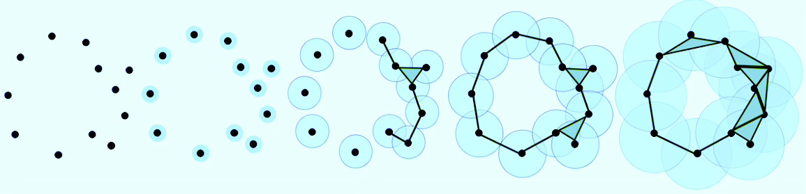
Topological Data Analysis (TDA) is a methodology that applies concepts from algebraic topology and computational geometry to analyze and extract meaningful patterns from complex datasets. It provides a geometric and topological perspective to study the shape and structure of data. TDA seeks to develop rigorous mathematical, statistical, and algorithmic techniques to infer, analyze, and leverage the intricate topological and geometric structures underlying data, often represented as point clouds in Euclidean or more general metric spaces [ref 50].
The most common topological domains are
Simplicial Complexes
Cellular Complexes
Hypergraphs
Combinatorial Complexes
In the simplest terms, a simplicial complex is a graph with faces. It generalizes graphs that model higher-order relationships among data elements—not just pairwise (edges), but also triplets, quadruplets, and beyond (0-simplex: node, 1-simplex: edge, 2-simplex: Triangle, 3-simplex: Tetrahedron, ) [ref 51].
You may wonder where simplicial complex fits in the overall picture of data representation.
💡 Laplacians & Graph Lifting
The following Laplacian matrices generalize the graph Laplacian to higher-dimensional simplicial complexes. Their purposes are
Generalization of the diffusion & message passing scheme
Capture higher-order dependencies (Boundaries and Co-boundaries)
Support convolution operations in Spectral Simplicial Neural Networks
Encoding of topological features such holes or cycles.
The Upper-Laplacian (a.k.a. Up-Laplacian) is a key operator in simplicial homology and Hodge theory, defined for simplicial complexes to generalize the notion of graph Laplacians to higher-order structures. The Up-Laplacian captures the influence of higher-dimensional simplices (e.g., triangles) on a given k-simplex. It reflects how k-simplices are stitched together into higher-dimensional structures.
The Down-Laplacian (a.k.a. Low-Laplacian) is similar to the Up-Laplacian except that the boundary operator projects k-simplices to (k-1) faces.
The Hodge Laplacian for simplicial complexes is a generalization of the graph Laplacian to higher-order structures like triangles, tetrahedra, etc. It plays a central role in topological signal processing, Topological Deep Learning, and Hodge theory. It is the sum of Up and Down Laplacian [ref 52].
🤖 For math-minded readers
Node, edge and face representation (or embedding) generated through Hodge Laplacian and incidence matrices are very sparse.
Full Simplicial lifting assigns signal/features to faces or triangles. Partial Simplicial lifting uses topological domains in the message passing and aggregation only (e.g., L1 Hodge Laplacian). This article applies Partial Simplicial Lifting.
💡 Persistent Homology & Cohomology
Persistent homology captures the topological structure of data across different spatial resolutions. Features that remain stable over many scales are interpreted as genuine properties of the space, while short-lived ones are viewed as noise or artifacts [ref 53].
Chain complex is a sequence of abelian groups ⋯- d(n+1) → C(n) — d(n)→ C(n-1) —d(n-1)→ … with boundary maps satisfying d(n−1)∘d(n)=0. Cochain complex: the “opposite-direction” version ⋯- d(n-1) → C(n) — d(n)→ C(n+1) —d(n+1)→ … with d(n+1)∘d(n)=0; this duality mirrors covariant vs. contravariant behavior [ref 54].
A Cohomology from a cochain complex gives algebraic invariants of a space. Compared to homology, cohomology often carries additional structure (e.g., a graded-commutative ring via the cup product) and many versions arise by dualizing homology constructions. De Rham Cohomology measures the “holes” of a smooth manifold using differential forms. Two forms count as the same cohomology class if they differ by a derivative (an exact form) [ref 55].
Filtrations of a space across scales give rise to persistent homology, summarizing the birth and death of features; distances between summaries are stable under small perturbations.
💡 Homotopy
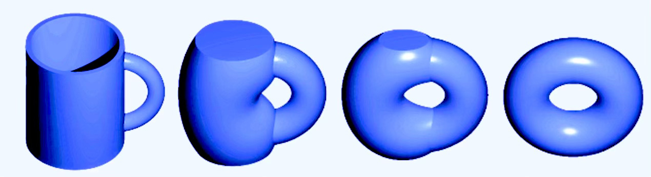
Homotopy theory is a branch of algebraic topology that studies the properties of spaces that are preserved under continuous deformations, called homotopies. It helps in distinguishing spaces that are topologically the same from those that are not and offers tools for working with complex spaces in mathematics and applied sciences [ref 56].
💡 Topological Deep Learning
Topological Deep Learning is widely considered a subfield of Geometric Deep Learning (GDL). Deep Learning distinguished by the way it defines local neighborhoods.
In geometric models built on continuous manifolds, the neighborhood around a point is typically represented by a local Euclidean space—often formalized as a tangent space or the Lie algebra at the identity of the manifold.
The distinction between Topological Data Analysis (TDA) and Topological Deep learning (TDL) can be confusing as both stem from algebraic topology.
While TDA supports analysis of the shape of input data (e.g., outliers, clusters,..), TDL is used to build learning models (e.g., Graph, Node, Simplex classification) that exploits both the input data and the output of TDA.
Applications
Molecular and protein modeling: Capture of 3D binding pockets, loops).
Mesh and 3D object analysis: Shape classification, segmentation
Sensor and communication networks: Detection of coverage holes and cycles
Neuroscience: Study of brain connectivity and functional cycles).
Point cloud data: Capture pf geometric and topological invariants).
Complex social and financial networks: Analysis of group interactions
…
🛠️ Python Libraries
TopoX
TopoX equips scientists and engineers with tools to build, manipulate, and analyze topological domains—such as cellular complexes, simplicial complexes, hypergraphs, and combinatorial structures—and to design advanced neural networks that leverage these topological components [ref 57].
The two packages we will leverage in future articles are
🔹 TopoNetX
An API for exploring relational data and modeling topological structures. It includes:
Atoms: Classes representing basic topological entities (e.g., cells, simplices)
Complexes: Classes for constructing and working with simplicial, cellular, path, and combinatorial complexes, as well as hypergraphs
Reports: Tools for inspecting and describing atoms and complexes
Algorithms: Utilities for computing adjacency and incidence matrices, and various Laplacian operators
Generators: Functions for creating synthetic topological structures
Installation
pip install toponetx🔹 TopoModelX
A library that provides template implementations for Topological Neural Networks. It supports applying convolution, message passing, and aggregation operations over topological domains.
Installation
pip install topomodelxGudhi
The GUDHI (Geometry Understanding in Higher Dimensions) library is an open-source framework focused on Topological Data Analysis (TDA), with a particular emphasis on understanding high-dimensional geometry [ref 58].
Similar to TopoX, it equips researchers with tools to construct and manipulate various complexes, including simplicial, cell, cubical, Alpha, and Rips complexes.
GUDHI supports the creation of filtrations and the computation of topological descriptors such as persistent homology and cohomology. Additionally, it offers functionality for processing and transforming point cloud data.
Installation
pip install gudhi📚 This Newsletter Articles
From Nodes to Complexes: A Guide to Topological Deep Learning
Exploring Simplicial Complexes for Deep Learning: Concepts to Code
Introduction to Geometric Deep Learning - Topological Models
Information-Geometric Learning
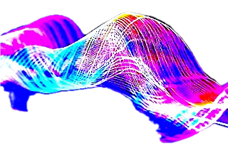
Information geometry applies differential-geometric tools to probability and statistics. It treats families of distributions as statistical manifolds—Riemannian manifolds whose points are probability laws—often equipped with a pair of conjugate affine connections; in many cases these structures are dually flat.
📌 I treat information geometry as distinct from differential geometry, much as I distinguish the natural gradient from the standard stochastic gradient. Other authors may differ.
Theory
💡Statistical manifolds
Information Geometry is derived from mathematical statistics and information theory [ref 59]. The well-known field of statistics covers discrete probability variables such as Binomial or Poisson distributions and probability density continuous functions such as Exponential or Gaussian distribution. Information theory pioneered by Claude Shannon owed its origin to thermodynamics and concern with the quantization of Entropy as a measure of the disorder (or chaos) in an irreversible system. The Gamma distribution plays a pivotal role in information theory.
Information geometry leverages Riemannian manifolds and metric, parallel transport, connection, tangent spaces, curvature and geodesics to extract geometric properties of various families of probability density functions [ref 60].
Statistical manifolds are smooth families of probability distributions represented as geometric, parameterized spaces.
💡 Fisher-Rao metric
The canonical Riemannian metric related to the distribution parameters is known as the Fisher-Rao metric or Fisher Information Matrix. Alongside of the Fisher-Rao metric, information geometry equips the manifold with two α-connections, known as dual affine connections: e-connection and m-connection. Parameters of exponential distributions are affine e-connections while expectation parameters are affine m-connection. Statistical manifolds can be induced with a Hessian metric for exponential distribution [ref 61, 62].
🤖 For math-minded readers
A Fisher-Riemann manifold is a differentiable manifold M whose points correspond to probability distributions p(x∣θ) from a statistical model parameterized by θ∈Θ⊂Rn, and which is equipped with the Riemannian metric g
The Fisher information metric for a continuous probability density function p is defined (outer product formulation).
Given that the expectation and differentiator operators can be interchanged. the metric can also be computed as (Hessian formulation)
💡Non-exponential Distributions
Information Geometry applies to Bivariate family of probability distribution such as McKay Bivariate Gamma and LogGamma manifold, Freund Bivariate Exponential and LogExponential manifold and Bivariate Gaussian manifold.
Information geometry extends spatial stochastic (Poisson) processes
💡Divergences
Kullback–Leibler (KL) divergence—a.k.a. relative entropy—measures how one probability distribution departs from a reference/target distribution. It’s not a metric (it’s asymmetric and fails the triangle inequality).
Jensen–Shannon (JS) divergence—the symmetrized, KL-based measure—quantifies similarity between two distributions and has a closed form for Gaussian families.
Bregman divergence (or Bregman “distance”) is a difference measure generated by a strictly convex function. When points represent probability distributions (e.g., model parameters or datasets), it serves as a statistical divergence. A basic example is squared Euclidean distance.
Applications
Neural network training: Stability using Natural Gradient.
Reinforcement learning: Application of Natural Policy Gradient and exponential distributions.
Manifold learning: Fisher-Rao geodesics to compute statistical distances.
Kullback-Leibler divergence: Minimization using information projection on manifolds.
Computer vision: Embedding distribution and covariance pooling.
Metric learning: Information geometric distances such as Log-Euclidean or Affine-Invariance metrics.
Uncertainty estimation: Fisher-Rao metric and Wasserstein distance.
Natural/Jeffrey priors: Fisher information geometry.
Variational Autoencoder: Statistical manifold representation of latent space.
Regularization: Fisher Information Matrix
Support Vector Machines: Information-geometric kernels
…
🛠️ Python Libraries
Information geometry is an extension of differential geometry, therefore the list of recommended Python libraries recommended for Manifold & Group-Based Learning -applies: Geomstats and Pymanopt
📚 This Newsletter Articles
📚 Abridged Glossary
α-connections: Dual pair of affine connection on a statistical manifold such as exponential family, with respect of the Fisher-Rao metric. Amari -1 connection is referred as m-connection and +1 connection as e-connection.
α-divergence: A particular type of f-divergence related to dual connection.
∇-affine coordinates: Affine e-connection or m-connection in which a local charts has null Christoffel symbols and geodesics are straight lines.
Barcode: A multi-set of intervals that records when topological features appear and disappear along a filtration in persistent homology.
Betti number: distinction of topological spaces based on the connectivity of n-dimensional simplicial complexes.
Bregman divergences: A class of distance-like functions that generalize the squared Euclidean distance using a convex function.
Cellular complex: A space built by gluing together basic building blocks called cells that objects homeomorphic to open shapes such as polygons, solids..
Centrality: Number or rankings of nodes within a graph that corresponds to their position. The list of types of centrality includes betweenness centrality, eigenvector centrality, degree centrality, closeness centrality and page rank.
Chain map: A map between chain complexes of modules is a sequence of module homomorphisms
Cohomology: A way to measure the global shape of a space using functions on elements rather than the elements themselves.
Combinatorial complex: Encode arbitrary set-like relations between collections of abstract entities. It permits the construction of hierarchical higher-order relations, analogous to those found in simplicial and cell complexes
Deformation (scaling, stretching, bending,….): A signal defined on a geometric domain (like a graph, manifold, or group) changes under transformations of that domain.
Deformation stability: A model’s ability to remain robust to small, non-structured distortions in the input in the context of equivariance
De Rham cohomology: Cohomology of complex of differential forms (smooth manifolds)
Diffusion on manifolds: Models designed for data constrained to lie on spheres, Lie groups, or statistical manifolds.
Directional derivative: Measures a function change as you move in a specific direction.
Domain deformation: A transformation or distortion of the geometric structure (domain) on which signals are defined.
Dual geometry: Pair of connection and conjugate connection related to dually flat manifolds.
e/m geodesic: Curves on e-connection or m-connection which coordinates are linear along the geodesic.
Equivariant neural network: A network that respects the symmetries of the input data.
Erdős–Rényi: Model for which all graphs on a fixed vertex set with a fixed number of edges are equally likely
Exponential map: A map from a subset of a tangent space of a Riemannian manifold.
f-divergences: A large family of statistical distance between probability distribution defined from a convex function. Kullback-Leibler and Jensen-Shannon are the most well-known statistical distances.
Filtration: A nested family of spaces indexed by a parameter so that earlier sets are contained in later ones. It is a sequence of subcomplexes for finite simplicial complex
Fisher–Rao metric (also referred as the Fisher information matrix): A Riemannian metric defined on a statistical manifold, which is a smooth space where each point corresponds to a probability distribution.
Flow matching: A generative modeling technique is to learn a transformation (or flow) that maps a simple base distribution (like a Gaussian) to a complex target distribution.
Gauge: A local choice of frames or coordinates used to describe geometric objects, particularly when those objects are defined on fiber bundles.
Geodesics: Curves on a surface that only turn as necessary to remain on the surface, without deviating sideways.
Graph cut: A partition of the vertices of a graph into two disjoint subsets.
Graph equivariance: A form of symmetry for functions from one graph with symmetry to another graph.
Graph isomorphism: A bijection between the vertex sets of two graphs. This is an equivalence relation used to categorize graphs.
Graph Laplacian: An operator in spectral graph theory that encodes the structure of a graph and is widely used in graph neural networks.
Graph path: A path in a graph is a finite or infinite sequence of edges which joins a sequence of vertices which are all distinct.
H-invariants such as H0 (components), H1 (rings) and H2 (voids) support persistence entropy and therefore dimension reduction for shape, molecules and regime change in time series.
Heat kernel: Solution to the heat equation with appropriate boundary conditions. It is used in the spectrum analysis of the Laplace operator.
Hodge–Laplacian: Canonical Laplace operator on differential k-forms on a Riemannian manifold.
Homeomorphism: A bijective map between topological spaces that is continuousand whose inverse is also continuous
Homogeneous space: A manifold on which a Lie group acts transitively.
Homophily: Property for which nodes with the same label or attributes are more likely to be connected in the network.
Homotopy: Ability for two continuous maps can be deformed into each other without tearing.
Hypergraph: Graph that supports arbitrary set-type relations without the notion of ranking.
Itakura-Saito divergence: A measure of the difference between a Spectrum (frequency) and its approximation. This is a type of Bregman divergence.
Killing field: A vector field on a pseudo-Riemannian manifold that preserves the metric tensor. The Lie derivative with respect of the field is null.
Laplace-Beltrami operator: Operator using second order derivative to quantify the curvature in a data manifold using a Riemannian metric.
Legendre-Fenchel transformation: Generalization of the Legendre transform to affine spaces that defines a convex conjugate.
Lie algebra: A vector space over a base field along with an operation locally called the bracket or commutator that satisfy bilinearity, Anti-symmetry and Jacobi Identity.
Lie-equivariant networks: Neural networks that are equivariant to transformations from a Lie group, such as rotations, translations, scaling, or Lorentz transformations.
Lie group: A differentiable space that is itself a group, meaning it supports smooth multiplication and inversion.
Logarithm map: A fundamental tool that translates points on a manifold back to the tangent space at a base point, typically to linearize the geometry for computation or analysis.
Manifold: A topological space that, around any given point, closely resembles Euclidean space.
Meshes: Structured collections of vertices, edges, and faces that together define the surface of a 3D object and encode explicit topological relationships between elements.
Natural gradient, NG: An optimization method that adapts the standard gradient by accounting for the geometry of the parameter space representing probability distributions.
Network flow: A graph with numerical capabilities on its edges
Network flow problem: Types of numerical problem in which the input is a flow defined as numerical values on a graph edges.
Neural operators: A class of machine learning models that learn mappings between infinite-dimensional function spaces.
Olliver-Ricci curvature: A notion of (coarse) Ricci curvature defined on any metric measure space using optimal transport. It is a key concept in discrete manifolds.
Persistent homology: Tracks topological features across different scales. It captures higher-order structural features such as holes, cycles and cavities
Persistent diagram: An alternative to visualize persistence homology. It is a summary of how topological features appear and disappear across a filtration.
Point cloud: A fundamental representation for real-world 3D data, especially when acquired via sensors.
Quantum groups: Mathematical structures that generalize Lie groups and Lie algebras, particularly in the context of non-commutative geometry and quantum physics.
Quiver: A directed graph where loops and multiple arrows between two vertices are allowed.
Random walk: A stochastic process that describes a path that consists of a succession of random steps on a graph.
Ricci curvature: A measure of how much the geometry of a manifold deviates from ‘being flat’, focusing on how volume or distance between geodesics changes.
Riemannian manifold: A differential manifold that comes with a metric tensor, providing a way to measure distances and angles
Riemannian metric: Assigns to each point a positive-definite symmetric bilinear form (e.g. dot product) to a manifold in a smooth way. This is a special case of metric tensor.
Set (a.k.a. category Set). A category with sets as object and function between sets as morphisms
Simplicial complex: A structured set of simplices (points, edges, triangles, and their n-dimensional analogues) in which every face of a simplex and every intersection of simplices is itself included.
Simplicial manifold: A simplicial k-complex that is homeomorphic to the link of every vertex looks like a (k-1) dimensional sphere.
Smooth or Differentiable manifold: A type of manifolds with a local differential structure, allowing for definitions of vector fields or tensors that create a global differential tangent space.
Spatial encoding: Spatial information such as related to curvature used as features of node or edges.
Spectral analysis: Study of the properties of a graph in relationship to its adjacency matrix and Laplacian matrix
Spectral convolution: Transformation of a signal into the frequency domain using the Laplacian eigenfunction basis, applying a spectral filter (pointwise multiplication), and transforming back.
Statistical manifold: Smooth manifolds in which each point represents a probability distribution, parameterized by one or more variables.
Stratified space: A space decomposed into smooth manifolds (called strata) arranged in a partially ordered fashion.
Tangent space at a point on a manifold: A set of tangent vectors at that point, like a line tangent to a circle or a plane tangent to a surface.
Topology-aware regularizers improves robustness against adversarial noise
Vietoris-Rips complex: A simplicial complex built from a metric space such as a point cloud using a distance threshold. It is analogous to a clique complex.
Von Mises-Fisher: A uniform random generator distributes data evenly across the hypersphere, making it unsuitable for evaluating k-Means.
Wasserstein distance: An optimal transport metric that measures how much work it takes to match the multiset of birth–death points from one persistent diagram to those of another.
Weisfeiler-Lehman: A graph test for the existence of an isomorphism between two graphs as a generalization of the color refinement algorithm.
🧠 Key Takeaways
✅ Geometric Deep Learning (GDL) takes symmetry as its organizing principle.
Symmetry can manifest as invariance—when something remains unchanged—or as equivariance—when it changes in a predictable way under transformation.
✅ Symmetry is a fundamental concept reflected throughout nature, geometry, shape, and mathematics
✅ This article breaks down Geometric Deep Learning into five key categories:
Graph Neural Networks, Mesh Modeling, Manifold & Group-Based Learning, Topological Deep Learning, and Information-Geometric Learning.
✅ GDL is supported by a rich ecosystem of Python libraries, including PyTorch Geometric, Geomstats, TopoX, and GUDHI, which make these geometric and topological principles practical for modern machine learning.
📘 References
A Brief Introduction to Geometric Deep Learning AI for Complex Data - J. McEwen - Medium, 2022
Geometric deep learning: going beyond Euclidean data M. Bronstein, J. Bruna, Y. LeCun, A. Szlam and P. Vandergheynst - 2017
Geometric foundations of Deep Learning - M. Bronstein - 2025
Geometric Deep Learning Book M. Bronstein, J. Bruna, T. Cohen, P. Veličković - 2021
Demystifying the Math of Geometric Deep Learning Hands-on Geometric Deep Learning - 2025
Mathematical Foundations of Geometric Deep Learning H. S. de Ocariz Borde, M. Bronstein - University of Oxford - 2015
A Practical Tutorial on Graph Neural Networks I. Ward, J. Joyner, C. Lickfold, Y. Guo, M. Bennamoun - 2012
Introduction to Graph Neural Networks: A Starting Point for Machine Learning Engineers - J. Tanis, C. Giannella, A. Mariano, The MITRE Corp. - 2024
A Comprehensive Introduction to Graph Neural Networks - Datacamp - 2022
Graph Neural Networks: A Gentil Introduction - YouTube. A. Persson - 2021
Stanford CS: Machine Learning with Graphs - YouTube - CS-224 Stanford University Online - 2022
Revisiting Inductive Graph Neural Networks Hands-on Geometric Deep Learning - 2025
Neighbors Matter: How Homophily Shapes Graph Neural Networks Hands-on Geometric Deep Learning - 2025
Introduction to Geometric Deep Learning - Graph Neural Networks Hands-on Geometric Deep Learning - 2025
Graph Theory Schaum’s Outlines - V. K. Balakrishnan, 1997
Introduction to Graph Theory Chap 1 Definition and Examples R. Wilson - 4th Edition - Addison-Wesley - 1996
An introduction to Graph Theory - Chap 3 Multigraphs D. Grinberg - Drexel University, Korman Center - 2025
Spectral Graph Theory D. Spielman - Yale University - 2011
Graph and Matrices - R. B. Bapat - Springer - 2009
PyTorch Geometric Documentation pyg.org
Taming PyTorch Geometric for Graph Neural Networks - Hands-on Geometric Deep Learning - 2025
Discrete Differential Geometry Series K. Crane - YouTube - 2021
Differential Geometric Approaches to Machine LearningA. Pouplin - DTU Library -2023
Introduction to Smooth Manifolds J. Lee - Springer Science+Business media New York - 2013
Differential Geometric Structures - W. Poor - Dover Publications, New York - 1981
Differential Geometry - From Elastic Curves to Willmore Surfaces - U, Pinkall, O. Gross - Compact Textbooks in Mathematics, Birkhauser - 2023
Riemannian Manifolds: Foundational Concepts - Hands-on Geometric Deep Learning - 2025
Differential Geometry - Tensor Calculus - R. Davie - YouTube - 2024
Differential Geometry - Khan Academy - YouTube - 2024
Tensor Analysis on Manifolds - Chap 5: Riemannian Manifolds R Bishop, S. Goldberg - Dover Publications, New York - 1980
Tensor Analysis on Manifolds - Chap 3: Vector Analysis on Manifolds R Bishop, S. Goldberg - Dover Publications, New York - 1980
Differential Geometric Structures- Chap 3: Riemannian Vector Bundles W. Poor - Dover Publications, New York - 1981
An Illustrated Introduction to the Ricci Flow G. Khan - 2022
Introduction to Lie Groups and Lie algebras Chap 1 & 2 - A Kirillov. Jr - SUNNY at Stony Brook - 2021
Lie groups & Lie algebras Series - J. Evans, YouTube - 2020
Lie Groups Beyond an Introduction - A. Knapp - 2023
SE(3): The Lie Group That Moves the World - Hands-on Geometric Deep Learning - 2025
Mastering Special Orthogonal Groups With Practice - Hands-on Geometric Deep Learning - 2025
geomstats: a Python Package for Riemannian Geometry in Machine Learning N. Miolane, J. Mathe, C. Donnat, M. Jorda, X. Pennec
Geomstats API GitHub
Pymanopt API GitHub
Exploring Geometric Learning with Geomstats - Hands-on Geometric Deep Learning - 2025
Topological Deep Learning: Going Beyond Graph Data - M. Hajij et all - 2023
An introduction to Topological Data Analysis: fundamental and practical aspects for data scientists - F. Chazal, B. Michel - 2021
Algebraic Topology for Data Scientists M. Postol - The MITRE Corporation, 2024
Topology - Chap 2: Elements of Point-Set Topology J. Hocking, G. Young - Dover Publications - 1988
Demystifying the Math of Geometric Deep Learning - Category Theory - Hands-on Geometric Deep Learning - 2025
Category Theory in Machine Learning - D. Shiebler, B. Gavranovic’, P. Wilson - University of Oxford, Strathclyde, Southampton - 2021
From Nodes to Complexes: A Guide to Topological Deep Learning - Hands-on Geometric Deep Learning - 2025
Exploring Simplicial Complexes for Deep Learning: Concepts to Code - Hands-on Geometric Deep Learning, 2025
Topological Lifting of Graph Neural Networks - Hands-on Geometric Deep Learning - 2025
A gentle introduction to persistent homology - C. Bock - 2019
Chain Complexes - MIT Libraries - 2021
Introduction to Differential Geometry Chap 6 De Rham Cohomology J. Robbin,
Topology - Chap 4: The Elements of Homotopy Theory J. Hocking, G. Young - Dover Publications - 1988
TopoX documentation - GitHub
GUDHI: Geometric Understanding of Higher Dimensions - INRIA, Fr
An Elementary Introduction to Information Geometry F. Nielsen - Sony Computer, 2 Science Laboratories, 2020
The Many Faces of Information Geometry F. Nielsen - Notices of the American Mathematical Society, 2022
What is Fisher Information? Ian Collings - YouTube, 2024
Shape your Model with Fisher-Rao Metric - Hands-on Geometric Deep Learning, 2025
Expertise Level
⭐ Beginner: Getting started - no knowledge of the topic
⭐⭐ Novice: Foundational concepts - basic familiarity with the topic
⭐⭐⭐ Intermediate: Hands-on understanding - Prior exposure, ready to dive into core methods
⭐⭐⭐⭐ Advanced: Applied expertise - Research oriented, theoretical and deep application
⭐⭐⭐⭐⭐ Expert: Research , thought-leader level - formal proofs and cutting-edge methods.
Share the next topic you’d like me to tackle.
Patrick Nicolas is a software and data engineering veteran with 30 years of experience in architecture, machine learning, and a focus on geometric learning. He writes and consults on Geometric Deep Learning, drawing on prior roles in both hands-on development and technical leadership. He is the author of Scala for Machine Learning(Packt, ISBN 978-1-78712-238-3) and the newsletter Geometric Learning in Python on LinkedIn.
++ Good Post, Also, start here how to build tech, Crash Courses, 100+ Most Asked ML System Design Case Studies and LLM System Design
How to Build Tech
https://open.substack.com/pub/howtobuildtech/p/how-to-build-tech-10-how-to-actually?r=14q3sp&utm_campaign=post&utm_medium=web&showWelcomeOnShare=false
https://open.substack.com/pub/howtobuildtech/p/how-to-build-tech-06-how-to-actually?r=14q3sp&utm_campaign=post&utm_medium=web&showWelcomeOnShare=false
https://open.substack.com/pub/howtobuildtech/p/how-to-build-tech-05-how-to-actually?r=14q3sp&utm_campaign=post&utm_medium=web&showWelcomeOnShare=false
https://open.substack.com/pub/howtobuildtech/p/how-to-build-tech-04-how-to-actually?r=14q3sp&utm_campaign=post&utm_medium=web&showWelcomeOnShare=false
https://open.substack.com/pub/howtobuildtech/p/how-to-build-tech-03-how-to-actually?r=14q3sp&utm_campaign=post&utm_medium=web&showWelcomeOnShare=false
https://open.substack.com/pub/howtobuildtech/p/how-to-build-tech-01-the-heart-of?r=14q3sp&utm_campaign=post&utm_medium=web&showWelcomeOnShare=false
https://open.substack.com/pub/howtobuildtech/p/how-to-build-tech-02-how-to-actually?r=14q3sp&utm_campaign=post&utm_medium=web&showWelcomeOnShare=false
Crash Courses
https://open.substack.com/pub/crashcourses/p/crash-course-09-part-1-hands-on-crash?utm_campaign=post-expanded-share&utm_medium=web
https://open.substack.com/pub/crashcourses/p/crash-course-07-hands-on-crash-course?utm_campaign=post-expanded-share&utm_medium=web
https://open.substack.com/pub/crashcourses/p/crash-course-06-part-2-hands-on-crash?utm_campaign=post-expanded-share&utm_medium=web
https://open.substack.com/pub/crashcourses/p/crash-course-04-hands-on-crash-course?r=14q3sp&utm_campaign=post&utm_medium=web&showWelcomeOnShare=false
https://open.substack.com/pub/crashcourses/p/crash-course-03-hands-on-crash-course?r=14q3sp&utm_campaign=post&utm_medium=web&showWelcomeOnShare=false
https://open.substack.com/pub/crashcourses/p/crash-course-02-a-complete-crash?r=14q3sp&utm_campaign=post&utm_medium=web&showWelcomeOnShare=false
https://open.substack.com/pub/crashcourses/p/crash-course-01-a-complete-crash?r=14q3sp&utm_campaign=post&utm_medium=web&showWelcomeOnShare=false
LLM System Design
https://open.substack.com/pub/naina0405/p/very-important-llm-system-design-577?utm_campaign=post-expanded-share&utm_medium=web
https://open.substack.com/pub/naina0405/p/very-important-llm-system-design-4ea?utm_campaign=post-expanded-share&utm_medium=web
https://open.substack.com/pub/naina0405/p/very-important-llm-system-design-499?r=14q3sp&utm_campaign=post&utm_medium=web&showWelcomeOnShare=false
https://open.substack.com/pub/naina0405/p/very-important-llm-system-design-63c?r=14q3sp&utm_campaign=post&utm_medium=web&showWelcomeOnShare=false
https://open.substack.com/pub/naina0405/p/very-important-llm-system-design-bdd?r=14q3sp&utm_campaign=post&utm_medium=web&showWelcomeOnShare=false
https://open.substack.com/pub/naina0405/p/very-important-llm-system-design-661?r=14q3sp&utm_campaign=post&utm_medium=web&showWelcomeOnShare=false
https://open.substack.com/pub/naina0405/p/very-important-llm-system-design-83b?r=14q3sp&utm_campaign=post&utm_medium=web&showWelcomeOnShare=false
https://open.substack.com/pub/naina0405/p/very-important-llm-system-design-799?r=14q3sp&utm_campaign=post&utm_medium=web&showWelcomeOnShare=false
https://open.substack.com/pub/naina0405/p/very-important-llm-system-design-612?r=14q3sp&utm_campaign=post&utm_medium=web&showWelcomeOnShare=false
https://open.substack.com/pub/naina0405/p/very-important-llm-system-design-7e6?r=14q3sp&utm_campaign=post&utm_medium=web&showWelcomeOnShare=false
https://open.substack.com/pub/naina0405/p/very-important-llm-system-design-67d?r=14q3sp&utm_campaign=post&utm_medium=web&showWelcomeOnShare=false
https://open.substack.com/pub/naina0405/p/most-important-llm-system-design-b31?r=14q3sp&utm_campaign=post&utm_medium=web&showWelcomeOnShare=false
https://naina0405.substack.com/p/launching-llm-system-design-large?r=14q3sp
https://naina0405.substack.com/p/launching-llm-system-design-2-large?r=14q3sp
[https://open.substack.com/pub/naina0405/p/llm-system-design-3-large-language?r=14q3sp&utm_campaign=post&utm_medium=web&showWelcomeOnShare=false
https://open.substack.com/pub/naina0405/p/important-llm-system-design-4-heart?r=14q3sp&utm_campaign=post&utm_medium=web&showWelcomeOnShare=false
https://open.substack.com/pub/naina0405/p/very-important-llm-system-design-63c?r=14q3sp&utm_campaign=post&utm_medium=web&showWelcomeOnShare=false
You identify inductive reasoning as the core gap LLMs deriving general laws from specific observations rather than pattern matching. I've been working on something that addresses this from the reasoning side rather than the architecture side. Not geometric priors baked in, not loss regularization, something that operates at inference time on unmodified models and appears to close some of that gap empirically. Tested it against published cybersecurity benchmarks with interesting results. Curious whether you think the architecture is the only viable path to genuine reasoning, or whether the reasoning process itself is addressable independently.