

Exploring Simplicial Complexes for Deep Learning: Concepts to Code
Expertise Level ⭐⭐⭐⭐

Does modeling your data with only nodes and edges feel limiting? Simplicial complexes offer a powerful alternative by capturing higher-order relationships among features, enabling more expressive and accurate models.
🎯 Why this matters
Purpose: While Graph Neural Networks (GNNs) have achieved notable success in modeling relational data through pairwise connections, they fall short in capturing higher-order interactions—essential for understanding complex systems such as protein folding, brain connectivity, physics-based models, energy networks, and traffic or flow dynamics.
Audience: Data scientists and engineers involved in Topology Data Analysis or developing deep learning models in non-Euclidean space such as Graph Neural Networks.
Value: .Learn how to represent graph-structured data as simplicial complexes through the use of incidence and Laplacian matrices.
🎨 Modeling & Design Principles
Overview
This article is a follow-up to our introduction to Topological Deep Learning in this newsletter [ref 1].
Graph Neural Networks (GNNs) have shown impressive success in handling relational data represented as graphs—mathematical structures that capture pairwise relationships through nodes and edges [ref 2, 3]. In contrast, Topological Deep Learning (TDL) extends this framework by incorporating more general abstractions that model higher-order relationships beyond simple pairwise connections.
⚠️ This article assumes a basic understanding of Geometric Deep Learning and Graph Neural Networks. These concepts have been introduced in previous articles [ref 4, 5, 6]
Simplicial Complex
In the simplest terms, a simplicial complex is a graph with faces. It generalizes graphs that model higher-order relationships among data elements—not just pairwise (edges), but also triplets, quadruplets, and beyond (0-simplex: node, 1-simplex: edge, 2-simplex: Triangle, 3-simplex: Tetrahedron, ) [ref 7, 8].
⚠️ Terminology: I use ‘simplex’ to mean any element of a simplicial complex—vertices, edges, triangles, and tetrahedra. While ‘face’ is sometimes used loosely as a synonym for ‘simplex,’ in this newsletter a ‘face’ refers specifically to triangles and tetrahedra.
0-simplex = vertex or node
1-simplex = edge
2-simplex = triangle
3-simplex = tetrahedron
You may wonder where simplicial complex fits in the overall picture of data representation. Contrary to a Graph Neural Network, the update for a k-dimensional feature h in a simplicial network typically involves three components:
Self-update: Direct flow between different dimensions (e.g., a triangle passing a summary to its edges).
Down message: Information flowing through shared faces
Up message: Information flowing through higher-order inclusions
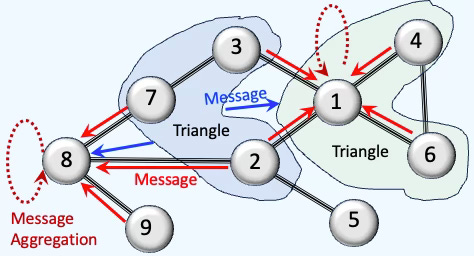
Fig. 1 Simplified overview of message passing in a simplicial neural network
It is useful to compare grid (node), graph (node + edge) and Simplicial complex (node + edge + triangle) to illustrate the increasing complexity of message passing as illustrated below.
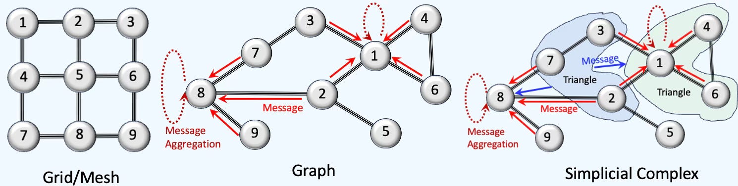
Fig. 2 Overview of Euclidean vs. Non-Euclidean data representation & message passing
Simplicial complex are usually associated with the analysis of shape in data, field known as Topological Data Analysis (TDA) [ref 9]
📌 Throughout this newsletter, I use the term “node”, which is commonly used to describe a vertex in a graph, although in academic literature you may also encounter the term “vertex” used interchangeably.
The following diagram illustrates a 7-nodes simplicial complex with 5 overlapping faces (4 triangles + 1 tetrahedron).
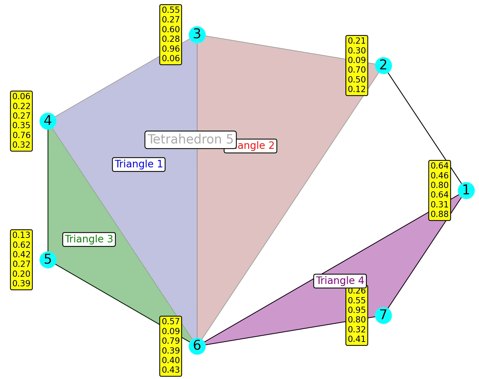
Fig. 3. Illustration of a 7-nodes, 8-edges, 4-triangles and 1-tetrahedron simplicial complex
⚠️ For convenience, we arbitrarily assign node indices starting at 1. This convention is followed for all the articles related to Topological Deep Learning.
Incidence/Boundary Matrices
Incidence vs Boundary Matrix
A common confusion is between incidence and boundary matrices. Boundary matrices encode the boundary operator with entries ±1 set by the relative orientation of faces; incidence matrices ignore orientation and use 0/1 only.
⚠️ You may find boundary vs. incidence matrix used interchangeably in the literature, including this newsletter.
Adjacency
This representation of graph is universally used to represent the relation between graphs. Here is an illustration of a simple simplicial complex of 5 nodes, 5 edges and 1 face.
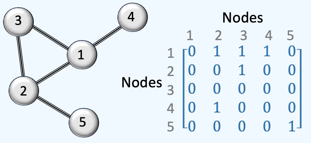
Fig. 4 Illustration of adjacency representation of a 5-nodes graph
Incidence Rank 0-2
The Incidence/Boundary Matrix specifies encoding of relationship between a k-dimensional and (k-1) -dimensional simplices (nodes, edges, triangle, tetrahedron,) in a simplicial complex.
Rank 0: The incidence/boundary matrix of rank 1 is simply the list of node indices
Rank 1: The rank-1 matrix for directed edges is computed as.
Here is an illustration of a simple simplicial complex of 5 nodes, 5 edges and 1 face.
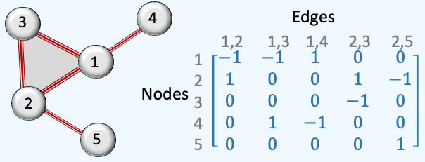
Fig. 5 Illustration of rank-1 boundary matrix of a 5-nodes simplicial complex
Rank 2: For a face [xi, xj, xk] with nodes xi, xj and xk and edges [xi, xj], [xi, xk] and [xj, xk
The incidence matrix is defined as
There is only one column in the matrix because there is only one face (red).
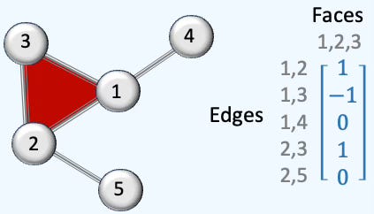
Fig. 6 Illustration of rank-2 boundary matrix of a 5-nodes, 1-face simplicial complex
The only column of is related to only face (1, 2, 3). The edges incident to face are (1, 2), (1, 2) and (2, 3), corresponding to the elements in the first, second and fourth row.
Simplicial Laplacians
The following Laplacian matrices generalize the graph Laplacian to higher-dimensional simplicial complexes. Their purposes are
Generalization of the diffusion & message passing scheme
Capture higher-order dependencies (Boundaries and Co-boundaries)
Support convolution operations in Spectral Simplicial Neural Networks
Encoding of topological features such holes or cycles.
The ranking of Laplacian reflects the complexity or dimension of the topological element from node, edges to faces as illustrated below:
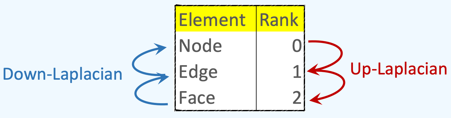
Fig. 7 Visualization of Up & Down-Laplacian for simplicial complexes
The difference between signed and unsigned Laplacians in the context of Simplicial Complexes lies in how orientation and directionality are treated in the boundary operators and, consequently, in the message passing behavior of Simplicial Neural Networks (SNNs).
A signed Laplacian preserves the orientation in the simplex while unsigned Laplacian does not.
📌 Signed Laplacians encode the structure (edges + faces) and orientation of boundaries. Unsigned Laplacians encode only the structure.
Upper-Laplacian
The Upper-Laplacian (a.k.a. Up-Laplacian) is a key operator in simplicial homology and Hodge theory, defined for simplicial complexes to generalize the notion of graph Laplacians to higher-order structures.
The Up-Laplacian captures the influence of higher-dimensional simplices (e.g., triangles) on a given k-simplex. It reflects how k-simplices are stitched together into higher-dimensional structures.
The diagonal of the matrix describes how many faces are incident to that edge aka the degree of that edge.
Its formal, mathematical definition is
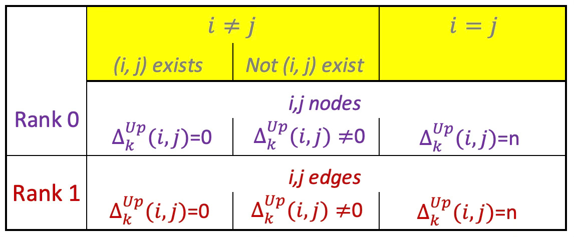
Table 1 Values of (i, j)th element of the Up-Laplacian of rank 0 and 1.
Down-Laplacian
The Down-Laplacian (a.k.a. Low-Laplacian) is similar to the Up-Laplacian except that the boundary operator projects k-simplices to (k-1) faces. It quantifies how k-simplex is influence by its lower-dimensional faces with the following mathematical definition:
From the formula it is obvious that the Down-Laplacian does not exist for rank 0 as the boundary would have rank -1!
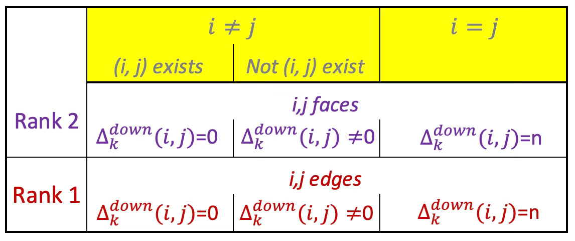
Table 2 Values of (i, j)th element of the Down-Laplacian of rank 1 and 2
The ranking Down-Laplacian of rank 0 does not make sense as the subelement of nodes does not exist.
Hodge-Laplacian
The UP and DOWN Laplacians we just introduced can be combined to generate the Hodge Laplacian. The Hodge Laplacian for simplicial complexes is a generalization of the graph Laplacian to higher-order structures like triangles, tetrahedra, etc. It plays a central role in topological signal processing, Topological Deep Learning, and Hodge theory.
The Hodge Laplacian plays a central role in Simplicial Neural Networks (SNNs) by enabling message passing across simplices of different dimensions (nodes, edges, faces, etc.), while preserving the topological structure of the data. .
For a simplicial complex, the Hodge Laplacian Δk at dimension k is defined as:
The Hodge Laplacian is a symmetric, positive semi-definite, square matrix with number of k-simplices as dimension. The Hodge Laplacian captures the flow of signals on a simplicial complex at various dimensions that is applicable to signal smoothing on higher-order domains.
Taking into account the existing constraints on the Up- and Down-Laplacian, the formulation of the Hodge-Laplacian can be simplified as follows:
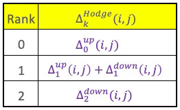
Table 3 Computation of the (i, j)th matrix element Hodge-Laplacian for rank 0, 1, & 2
⚙️ Hands‑on with Python
Environment
Libraries: Python 3.12.5, PyTorch 2.5.0, Numpy 2.2.0, Networkx 3.4.2, TopoNetX 0.2.0
Source code is available at
Features: geometriclearning/topology/simplicial/featured_simplicial_complex.py
Evaluation: geometriclearning/play/featured_simplicial_complex_play.py
The source tree is organized as follows: features in python/, unit tests in tests/, and newsletter evaluation code in play/.
To enhance the readability of the algorithm implementations, we have omitted non-essential code elements like error checking, comments, exceptions, validation of class and method arguments, scoping qualifiers, and import statements.
We rely on Python libraries TopoX and NetworkX introduced in a previous article [ref `10, 11].
NetworkX is a BSD-license powerful and flexible Python library for the creation, manipulation, and analysis of complex networks and graphs. It supports various types of graphs, including undirected, directed, and multi-graphs, allowing users to model relationships and structures efficiently [ref 12]
TopoX equips scientists and engineers with tools to build, manipulate, and analyze topological domains—such as cellular complexes, simplicial complexes, hypergraphs, and combinatorial structures—and to design advanced neural networks that leverage these topological components [ref 13]
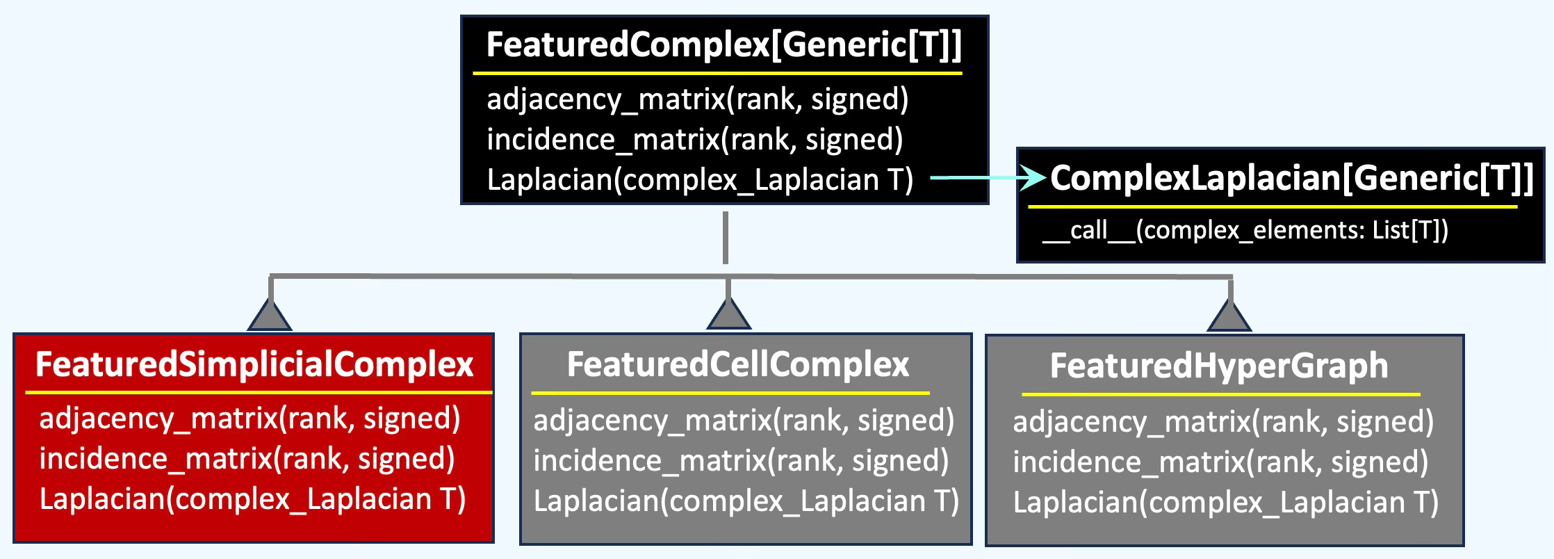
👉 We unify the functionality of multiple topological domains—Simplicial Complexes, Cell Complexes and Hypergraph—within a class hierarchy to enable systematic comparison of their behavior, from incidence matrices to Hodge Laplacians.
Setup
We define a simplicial element as a node, edge, face (triangle or tetrahedron). A simplicial element is defined by its
features: An optional feature vector
simplex_indices: List of indices of nodes composing the simplicial element. A node has a single index, edge two, a triangle 3 and a tetrahedron 4.
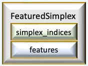
Fig. 8 Illustration of components of a featured simplex
The list of indices of nodes is an implicit ordered list of indices starting with 1. As with graph a list of nodes indices defined as tuple (node source, node target) (e.g., [[1, 2], [1,3], [2, 4], …]).
A feature vector is potentially associated with each of the simplicial element (node, edge and faces) as illustrated below:
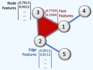
Fig. 9 Illustration of feature vector associated with each simplicial element.
📌 The feature vector on edge and faces is not strictly required. In this scenario, the simplicial complex acts as a standard graph.
🔎 Simplicial Elements
Any topological deep learning model relies on features defined on nodes, edges and higher-order constructs such as faces. Therefore, we associated an optional feature vector to a cell element as a node, edge, polygon. A featured cell element is defined by its
features: An optional feature vector associated with a cell
cell: A cell with elements (indices) and rank
📌 TopoNetX allows to assign feature keys and values to each individual cell is similar to creating a key-value pair in a dictionary as described in Graph Reimagined: The Power of Cell Complexes - Featured Cell
Firstly, let’s create a class, FeaturedSimplex to define the basic component of the Simplicial Complex as described in the previous section (code snippet 1).
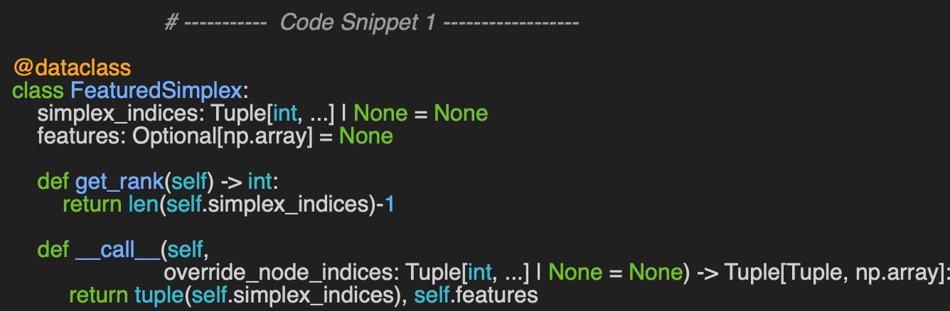
The two attributes are
simplex_indices: Indices of nodes defining the simplex (e.g., edge = (3, 6))
features: The feature vector implemented as a Numpy array
The __call__ method initializes if needed or update the simplex indices
For sake of convenience, we wrap the configuration and operation on simplicial complex into a class FeaturedSimplicialComplex which implements the attributes and operations on simplicial complexes.
The constructor has 1 argument (code snippet 2), features_simplices which is list of FeaturedSimplex instances (simple node indices and feature vectors)
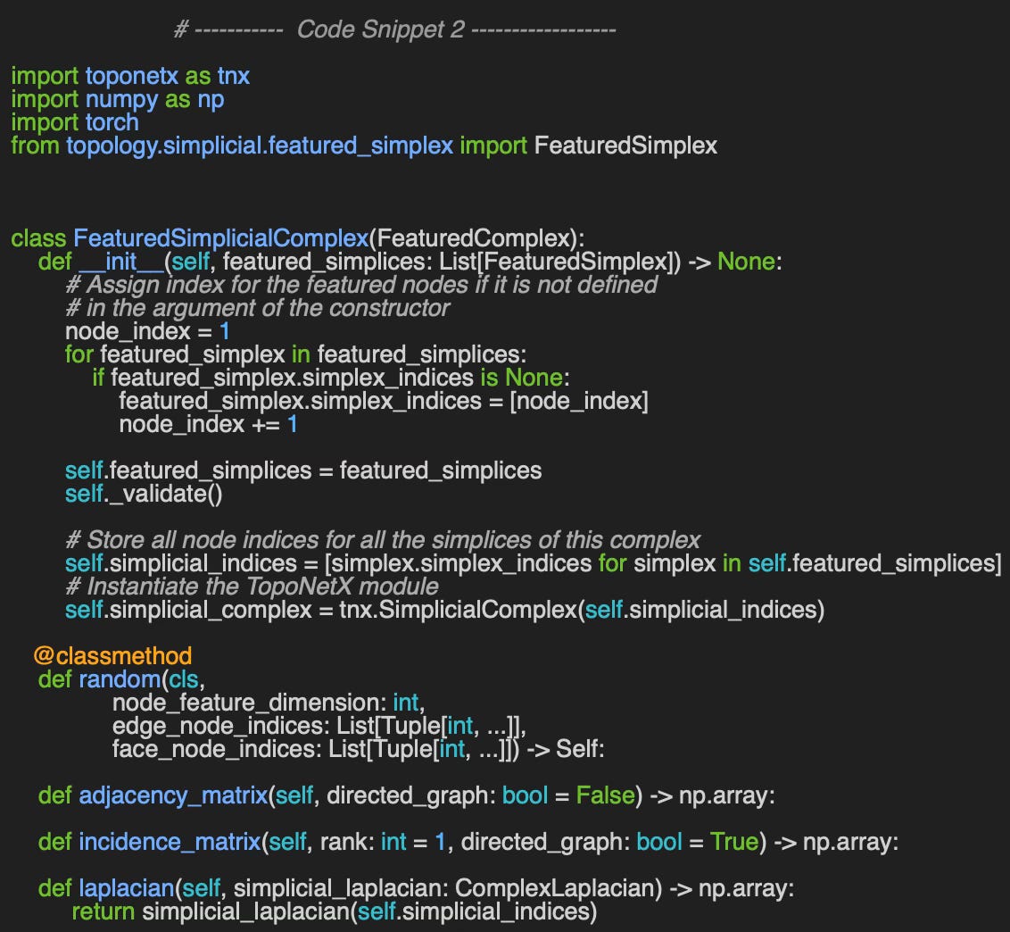
The methods adjacency_matrix, incidence_matrix and laplacian will be described in the subsequent sections.
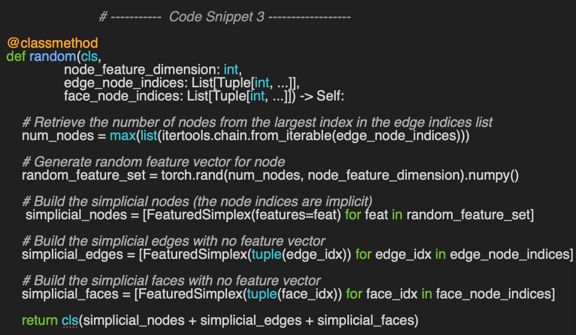
For evaluation or illustration purpose we do not need to provide a graph dataset with feature vector for each of the simplicial element (node, edge or faces). To this purpose, we implement an alternative constructor, random that generates random features vectors for node only with the appropriate node_feature_dimension. I leverage the itertools package to extract the largest node index.
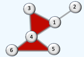
Let’s consider a 5 nodes, 5 edges, 2 triangles simplicial complex with the following configuration:
edge_set = [[1, 2], [1, 5], [2, 3], [2, 4], [3, 4], [2, 5], [4, 5]]
face_set = [[4, 2, 3], [2, 4, 5]]
with 6-feature vector/node and displayed using NetworkX library
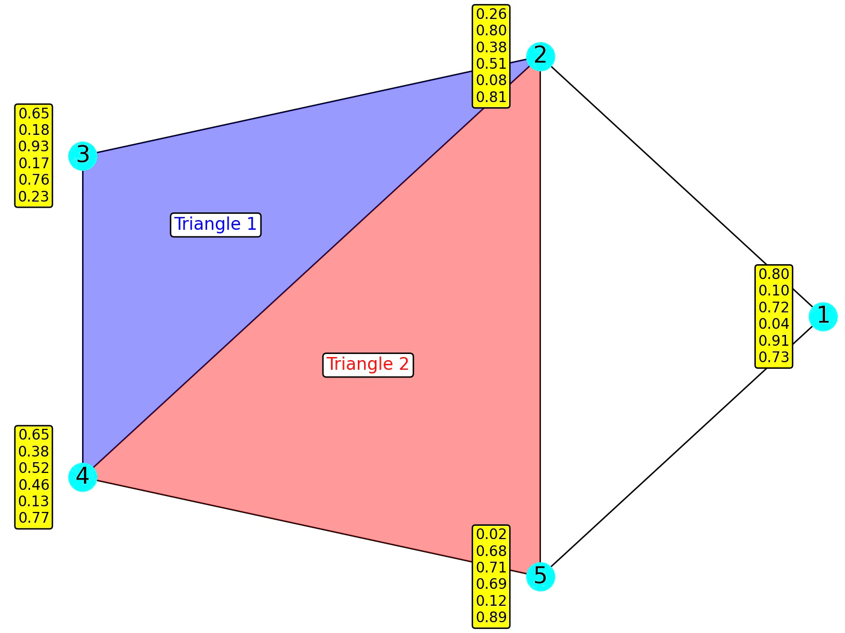
Fig. 10 Visualization of the test graph data used computing incidence and Laplacian matrices
This configuration is used for the rest of the article to compute incidence matrices and various Laplacian.
🔎 Incidences
Let’s look like an unusual implementation of the adjacency matrix, adjacency_matrix for the fun of it! The boolean flag, signed specifies if the graph is directed or undirected to enforce symmetry if necessary (code snippet 4).
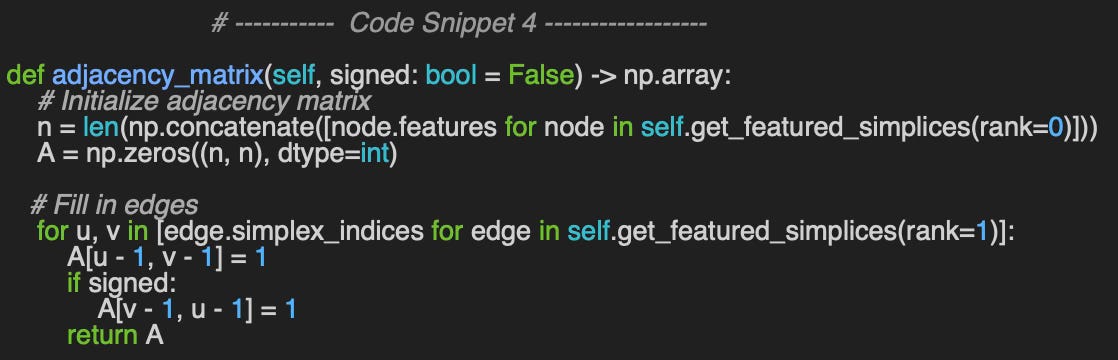
👉 The test code: geometriclearning/play/featured_simplicial_complex_play.py
We need to choose a dataset for our simplicial complex that is realistic enough to reflect practical scenarios, yet simple enough to avoid confusing the reader when implementing various operators (code snippet 5).
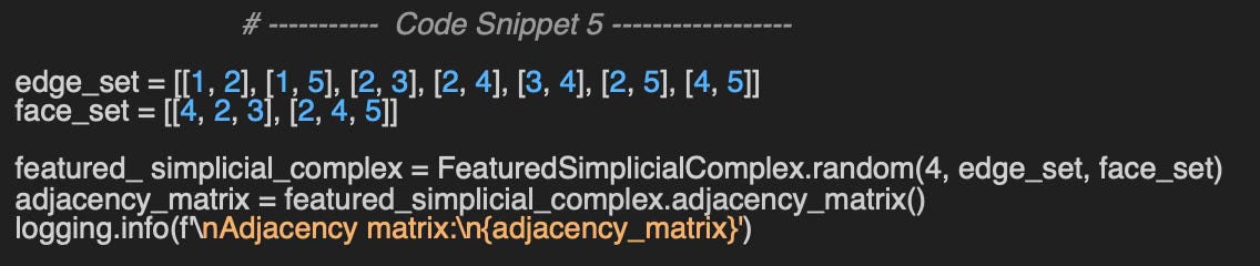
Output:
Adjacency matrix:
[[0 1 0 0 1]
[0 0 1 1 1]
[0 0 0 1 0]
[0 0 0 0 1]
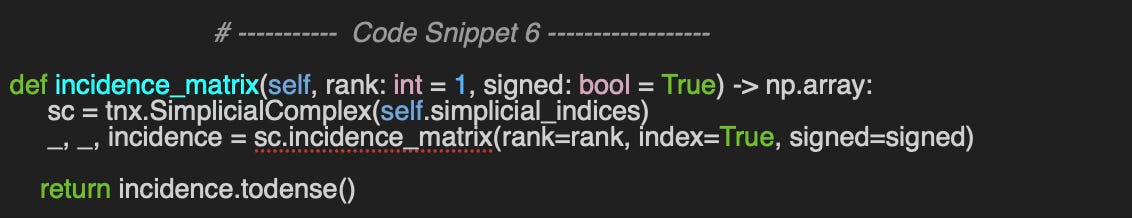
[0 0 0 0 0]]The incidence matrices are a bit more complex as they create a representation of faces from edges (columns) and nodes (rows). Once again, the implementation incidence_matrix method of FeaturedSimplicialComplex class leverages the TopoNetX package.
We compute the incidence of rank 1 and 2 on the same graph set defined in code snippet 5.
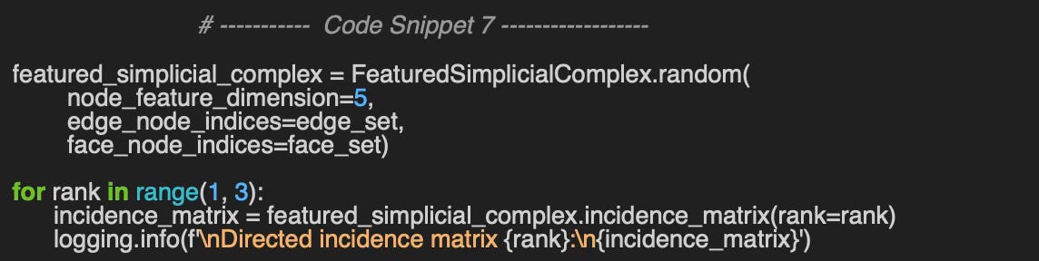
Output:
Directed incidence matrix 1:
[[-1. -1.  0.  0.  0.  0.  0.]
 [ 1.  0. -1. -1. -1.  0.  0.]
 [ 0.  0.  1.  0.  0. -1.  0.]
 [ 0.  0.  0.  1.  0.  1. -1.]
 [ 0.  1.  0.  0.  1.  0.  1.]]

Directed incidence matrix 2:
[[ 0.  0.]
 [ 0.  0.]
 [ 1.  0.]
 [-1.  1.]
 [ 0. -1.]
 [ 1.  0.]
 [ 0.  1.]]
🔎 Laplacians
The computation of the various Laplacian is implemented by the method laplacian of class AbstractSimplicialComplex. This method invokes the Laplacian configuration data class SimplicialLaplacian.
This class serves as a simple wrapper for the different types of Laplacians supported by the TopoX library.
The configuration includes the following parameters (code snippet 8).
simplicial_laplacian_type: An enumerated type indicating the kind of Laplacian to compute — Up-Laplacian, Down-Laplacian, or Hodge Laplacian.
rank: Specifies the rank at which the Laplacian is applied — 0 or 1 for Up-Laplacian, 1 or 2 for Down-Laplacian, and 1, 2, or 3 for Hodge Laplacian.
signed: A boolean flag that determines whether the Laplacian is directed (signed) or undirected.
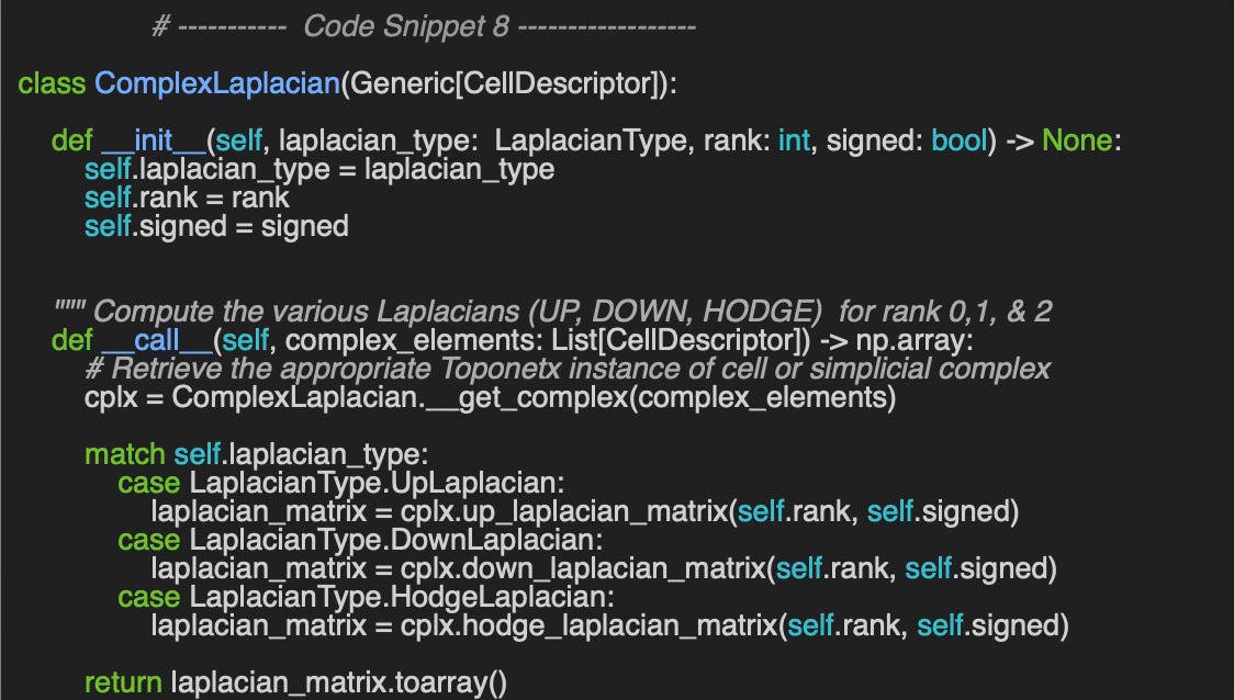
📌. The order in the list of edge indices and face indices, edge_set and face_set is specified does not affect the computation Laplacian matrices
🔎 Up-Laplacian rank 0, 1
The following code snippet compute the Up-Laplacian of Rank 0 (node & edges) and Rank 1 (edges & faces).
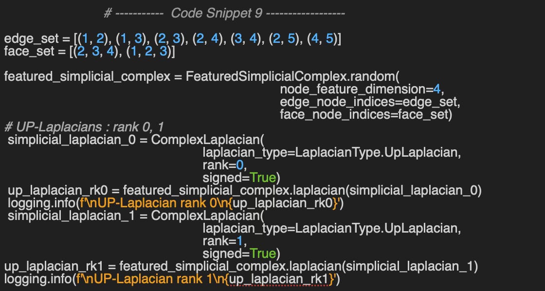
Output:
Up-Laplacian rank 0
[[ 2. -1.  0.  0. -1.] #Node1 to incidence edges (1,2),(1,5)
 [-1.  4. -1. -1. -1.] #Node2 to incidence edges (1,2,(2,3),(2,4),(2,5)
 [ 0. -1.  2. -1.  0.]
 [ 0. -1. -1.  3. -1.]
 [-1. -1.  0. -1.  3.]]
The Up-Laplacian of rank 0 searches for the node, retrieves its incident edges and compute the number of incident nodes associated with these edges.
Let’s understand the computation for a couple of rows in the Laplacian matrix.
Row 1: Node 1 has 3 incidence edges (1, 2) & (1, 5). Each edges related to nodes 1, 2, and 5 with value 2, -1 (inverted edge) & -1 (inverted edge). Values related to nodes 3 & 4 are obviously 0
Row 2: Node 2 has 5 incidence edges: (2, 1) = -(1, 2), (2, 3), (4, 2) = -(2, 4),.. The node is connected to each of all other 4 nodes 1, 3, 4 & 5. Therefore, the Laplacian value for (2, 2) is 4.
Up-Laplacian rank 1
[[ 0.  0.  0.  0.  0.  0.  0.]
 [ 0.  0.  0.  0.  0.  0.  0.]
 [ 0.  0.  1. -1.  0.  1.  0.] # Edge(2,3): incidences (4,2,3),
 [ 0.  0. -1.  2. -1. -1.  1.] # Edge(2,4): incidences(4,2,3),(2,4,5)
 [ 0.  0.  0. -1.  1.  0. -1.]
 [ 0.  0.  1. -1.  0.  1.  0.]
 [ 0.  0.  0.  1. -1.  0.  1.]]
Row 3: Edge (2, 3) has 1 incidence face (4, 2, 3). Each edge of the triangle (4, 2, 3), are (1, 2), (3, 2) = -(3, 3) & (3, 4).
Row 4: The 4rd edge (2, 4) is shared between the two faces/triangles (4, 2, 3) & (2, 4, 5) so the value of the Laplacian is 2. The two other edges of each triangle (4, 3), (2, 3) for the 1st triangle and (2, 5) and (4, 5) are not shared, therefore their Laplacian values is +/- 1.
Down-Laplacian rank 1, 2
The implementation for the Up-Laplacian can be easily modified to compute the Down-Laplacian for rank 1, 2 (code snippet 10).
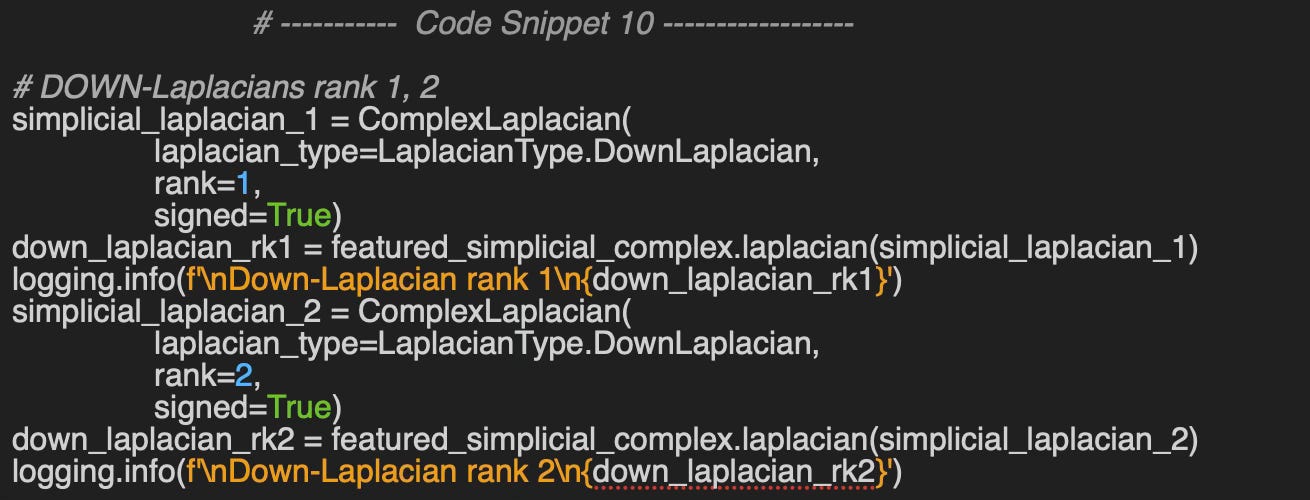
Rank 1 takes any of the edges, search for the incident nodes and computes the number of edges incident to these nodes.
Down-Laplacian rank 1
[[ 2.  1. -1. -1. -1.  0.  0.]
 [ 1.  2.  0.  0.  1.  0.  1.]
 [-1.  0.  2.  1.  1. -1.  0.]
 [-1.  0.  1.  2.  1.  1. -1.]
 [-1.  1.  1.  1.  2.  0.  1.]
 [ 0.  0. -1.  1.  0.  2. -1.]
 [ 0.  1.  0. -1.  1. -1.  2.]]
Rank 2 takes any of the faces, searches for the incident edges and computes the number of faces incident to these edges.
Down-Laplacian rank 2
[[3. 1.]
 [1. 3.]]
This Down-Laplacian matrix has 2 x 2 dimension as there are only 2 faces (1, 2, 3) & 2, 3, 4) with (2, 3) edge shared resulting in Laplacian value of 3.
Hodge-Laplacian rank 0, 1 & 2
As mentioned earlier, the Hodge Laplacian is defined as the sum of the Up-Laplacian and the Down-Laplacian, for all ranks where these matrices are defined
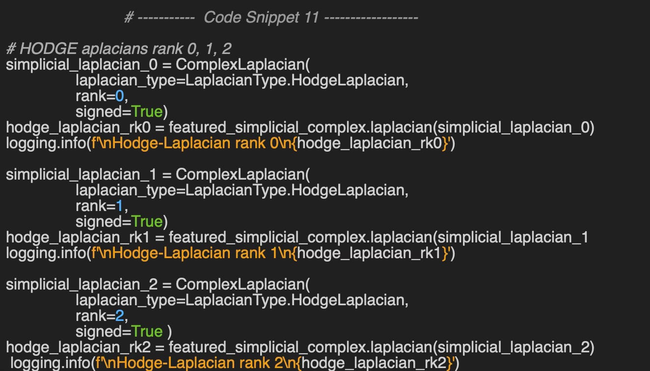
Output
Hodge-Laplacian rank 0
[[ 2. -1.  0.  0. -1.]
 [-1.  4. -1. -1. -1.]
 [ 0. -1.  2. -1.  0.]
 [ 0. -1. -1.  3. -1.]
 [-1. -1.  0. -1.  3.]]

Hodge-Laplacian rank 1
[[ 2.  1. -1. -1. -1.  0.  0.]
 [ 1.  2.  0.  0.  1.  0.  1.]
 [-1.  0.  3.  0.  1.  0.  0.]
 [-1.  0.  0.  4.  0.  0.  0.]
 [-1.  1.  1.  0.  3.  0.  0.]
 [ 0.  0.  0.  0.  0.  3. -1.]
 [ 0.  1.  0.  0.  0. -1.  3.]]

Hodge-Laplacian rank 2
[[3. 1.]
 [1. 3.]]
This test confirms that the rank-0 Hodge Laplacian is identical to the rank-0 Up-Laplacian computed in the previous test. Likewise, the rank-2 Hodge Laplacian matches the rank-2 Down-Laplacian.
More Examples
The library NetworkX is versatile enough [ref 14] that it allows us to draw few more elaborate simplicial complexes. The source code to visualize Simplicial complex is available at Github SimplicialFeatureSet.show
 edge_set = [
   [1, 2], [1, 3], [1, 6], [2, 3], [5, 3], [3, 6], [3, 4], [1, 7],
   [6, 7], [7, 8], [8, 9], [7, 9], [5, 6], [4, 5], [3, 6]
 ]

face_set = [
   [1, 2, 3], [5, 3, 6], [3, 5, 4], [1, 6, 7], [7, 8, 9], # Triangles'
   [5, 3, 6, 4]   # Tetrahedron
]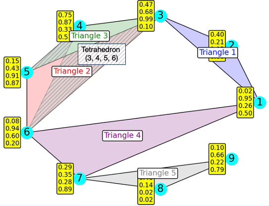
Fig. 11 Visualization of a 9 nodes, 15, edges, 6 Triangles, 1 Tetrahedron simplicial complex
edge_set = [
 [1, 2], [1, 3], [1, 6], [2, 3], [5, 3], [3, 6], [3, 4], [1, 7], [6, 7],
 [7, 8], [8, 9], [7, 9], [5, 6],[4, 5], [3, 6], [9, 10], [9, 7],
 [10, 11], [7, 11], [7, 10], [11, 12], [7, 12], [7, 13], [13, 14],
 [14, 15], [15, 16], [16, 17], [17, 18], [7, 14], [7, 16], [18, 19],
 [19, 20], [20, 21], [1, 16], [1, 17], [17, 21], [19, 21], [21, 22],
 [22, 23], [23, 1], [1, 21], [1, 22]
]

face_set = [
# Triangles
   [1, 2, 3], [5, 3, 6], [3, 5, 4], [1, 6, 7], [7, 8, 9], [7, 9, 10],
   [7, 10, 11], [7, 13, 12], [7, 14, 16], [7, 13, 14], [1, 16, 17],
   [17, 21, 19], [17, 21, 1], [21, 22, 1],
# Tetrahedrons
   [5, 3, 6, 4], [7, 9, 10, 11], [7, 13, 14, 16], [1, 17, 19, 21]
]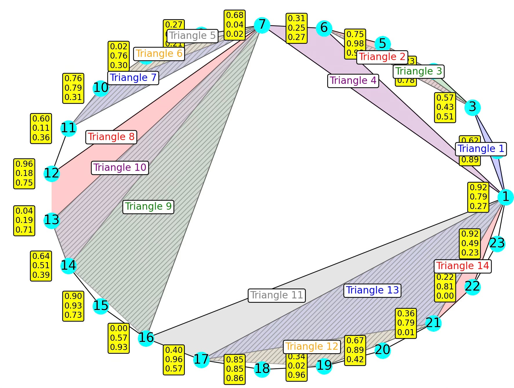
Fig. 12 Visualization of a 23 nodes, 42 edges, 14, triangles & 4 tetrahedron Simplicial Complex
🧠 Key Takeaways
✅ Simplicial complexes extend graphs by modeling higher-order relationships—not just pairwise interactions (edges), but also group interactions such as triangles and tetrahedra.
✅. The structure of a simplicial complex is captured by incidence matrices: rank-1 matrices describe connections between nodes and edges, while rank-2 matrices relate edges to faces.
✅ The Up-Laplacian, Down-Laplacian, and Hodge Laplacian generalize the traditional graph Laplacian, enabling message passing across simplices of different dimensions, encoding topological features, and capturing both boundaries and co-boundaries of faces.
✅ Together, the TopoX and NetworkX libraries offer scientists and engineers a powerful toolkit to construct, manipulate, and analyze simplicial complexes in data-driven applications.
📘 References
From Nodes to Complexes: A Guide to Topological Deep Learning Hands-on Geometric Deep learning - 2025
A Practical Tutorial on Graph Neural Networks I. Ward, J. Joyner, C. Lickfold, Y. Guo, M. Bennamoun
YouTube: Build your first GNN A. Nandakumar
Introduction to Geometric Deep Learning Hands-on Geometric Deep learning - 2025
Demystifying Graph Sampling & Walk Methods Hands-on Geometric Deep learning - 2025
Taming PyTorch Geometric for Graph Neural Networks Hands-on Geometric Deep learning - 2025
Topological Deep Learning: Going Beyond Graph Data M. Hajij et all
Architectures of Topological Deep Learning: A Survey on Topological Neural Networks M. Papillon, S. Sanborn, M. Hajij, N. Miolane
Introduction to Geometric Deep Learning: Topological Data Analysis P. Nicolas - Hands-on Geometric Deep learning
From Nodes to Complexes: A Guide to Topological Deep Learning - NetworkX
From Nodes to Complexes: A Guide to Topological Deep Learning - TopoX
TopoNetX Documentation - PyT-Team
Visualization of Graph Neural Networks P. Nicolas - LinkedIn Newsletter - 2025
🛠️ Q&A
Q1: Does the Down-Laplacian exist for rank-0 simplices? If so, what is its interpretation?
Q2: What is the rank-2 incidence matrix for the given simplicial complex?
Q3: How is the Hodge Laplacian computed from the Up- and Down-Laplacians?
Q4: How many different ranks (dimensions) can a Hodge Laplacian be defined for in a simplicial complex?
Q5: What are the key differences between signed and unsigned Laplacians?
Q6: How does the ordering of edge indices influence the computation of the Laplacians?
💬 News & Reviews
This section focuses on news and reviews of papers pertaining to geometric deep learning and its related disciplines.
Paper Review: Flow Matching on Lie groups F. Sherry, B. Smets - Dept. of Mathematics & Computer Science, Eindhoven University of Technology - 2025
Flow matching has been extensively explored in Euclidean spaces using linear conditional vector fields. However, extending this concept to Riemannian manifolds poses challenges. A natural idea is to replace straight lines with geodesics, but this often becomes intractable on complex manifolds due to the difficulty of computing geodesics under arbitrary metrics.
To address this, the authors propose an alternative approach based on Lie group exponential maps, which is particularly effective for Special Orthogonal (SO(n)) and Special Euclidean (SE(n)) groups, leveraging efficient matrix operations.
Their method approximates the vector field induced by a Riemannian metric using a neural network. The conditional vector field is guided by an exponential curve—i.e., the exponential map applied to a Lie algebra element derived from a group element at time tt.
The model is evaluated on SO(3), SE(2), product groups, and homogeneous spaces, demonstrating strong alignment between the learned and target distributions—especially when the exponential curves are not overly complex.
Notes:
Source code and animations are available on GitHub.
The paper assumes readers are familiar with differential geometry, Lie groups, and Lie algebras.
Expertise Level
⭐ Beginner: Getting started - no knowledge of the topic
⭐⭐ Novice: Foundational concepts - basic familiarity with the topic
⭐⭐⭐ Intermediate: Hands-on understanding - Prior exposure, ready to dive into core methods
⭐⭐⭐⭐ Advanced: Applied expertise - Research oriented, theoretical and deep application
⭐⭐⭐⭐⭐ Expert: Research , thought-leader level - formal proofs and cutting-edge methods.
Share the next topic you’d like me to tackle.
Patrick Nicolas is a software and data engineering veteran with 30 years of experience in architecture, machine learning, and a focus on geometric learning. He writes and consults on Geometric Deep Learning, drawing on prior roles in both hands-on development and technical leadership. He is the author of Scala for Machine Learning (Packt, ISBN 978-1-78712-238-3) and the newsletter Geometric Learning in Python on LinkedIn.