

Taming PyTorch Geometric for Graph Neural Networks
Expertise Level ⭐⭐

Overwhelmed by the functionality and complexity of the PyTorch Geometric API?
You're not alone. Since its introduction in early 2019 [Ref 1], PyTorch Geometric has expanded significantly, incorporating new models, graph samplers, and transformations, continuously evolving to align with the latest research publications.
This article marks the first installment in a series aimed at demystifying the full capabilities of PyTorch Geometric.

🎯 Why this Matters
Purpose: PyTorch Geometric has emerged as a leading library for exploring and implementing Graph Neural Networks (GNNs) using PyTorch. However, the vast array of available models and techniques can be overwhelming.
Audience: Data scientists and machine learning engineers seeking a library to develop models that capture complex relationships between entities.
Value: Gain a foundational understanding of PyTorch Geometric and learn how to efficiently navigate its diverse functionalities.
🎨 Modeling & Design Principles
Overview
The key Features of PyTorch Geometric are [ref 2]:
Efficient Graph Processing: Optimizes memory and computation using sparse graph representations.
Flexible GNN Layers: Covers GCN, GAT, GraphSAGE, GIN, and other advanced architectures.
Batching for Large Graphs: Supports for mini-batching for handling graphs with millions of edges.
Seamless PyTorch Integration: Provides full compatibility with PyTorch tensors, autograd, and neural network modules.
Diverse Graph Support: PyTorch Geometric handles directed, undirected, weighted, and heterogeneous graphs.
The most important PyG Modules are:
torch_geometric.data to manages graph structures, including nodes, edges, and features.
torch_geometric.nn to provide data scientists prebuilt GNN layers like convolutional and gated layers.
torch_geometric.transforms to pre-process input data (e.g., feature normalization, graph sampling).
torch_geometric.loader to handle large-scale graph datasets with specialized loaders.
📌 PyTorch Geometric, Torch Geometric and the abbreviation PyG refers to the same library. We will use these terms interchangeably.
Design Challenges
We've only scratched the surface when it comes to the complexities of configuring a Graph Neural Network. At a minimum, you need to consider several key components:
Graph Neural Model: Options include Graph Attention Network (GAT), Graph Sample and Aggregate (GraphSAGE), and Graph Convolutional Network (GCN).
Graph Data Loader: Works with samplers like GraphSAINTSampler and NeighborLoader.
Graph Convolution Layer: Tied to the model, such as GATConv, GraphConv or SAGEConv.
Aggregation Method: Choices include SumAggregation, MeanAggregation and MulAggregation.
Pooling Layer: Many options range from ClusterPooling and SAGPooling to MemPooling.
Transforms: Examples include NormalizeFeatures, RandomLinkSplit or SVDFeatureReduction .
… and many more! The challenge lies in selecting the right combination tailored to your dataset and task.
The Graph Convolutional Network chosen in the hands-on section highlights the challenges of configurability. Meanwhile, let's take a quick look at different Graph Neural Network models, datasets, and data loaders.
Graph Neural Networks
📌📌This section does not provide a theoretical review of Graph Neural Networks (GNNs), including node embeddings, permutation equivariance, message passing, or aggregation policies. Instead, there are numerous high-quality tutorials and detailed explanations available in both printed resources and online materials. I recommend the following references 3, 4, 5, & 6 as tutorial and 7 & 8 for foundational knowledge.
You may wonder where graph fits in the overall picture of complex data representation.
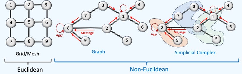
Fig. 1 Overview of Euclidean vs. Non-Euclidean Data Representation
What is a Graph Neural Network?
A Graph Neural Network (GNN) is an optimizable transformation on all attributes of the graph (nodes, edges, global context) that preserves graph symmetries (permutation invariances). GNN takes a graph as input and generate/predict a graph as output.
Data on manifolds can often be represented as a graph, where the manifold's local structure is approximated by connections between nearby points. GNNs and their variants (like Graph Convolutional Networks (GCNs) extend neural networks to process data on non-Euclidean domains by leveraging the graph structure, which may approximate the underlying manifold.
Scope
There are 3 types of tasks to be performed on a GNN:
Graph-level task: Predict the property of the entire graph such as classification problems with MNIST or CIFAR images or sentiment analysis for a document or paragraph.
Node-level task: Predict if a node belongs to a specific class (i.e. Karate club) or image segmentation (identify the role of a pixel in an image) or part of speech a word belongs to.
Edge-level task: Predict the relationship between node (i.e. Interaction between users) that can be classified (discovery of connections between entities or nodes). The task also consists in pruning a fully connected graph into a sparse graph.
Types
Application such as social network analysis, molecular structure prediction, and 3D point cloud data can all be modeled using GNNs. Here is an overview of the major types of GNNs:
Graph Convolutional Network (GCN): GCNs generalize the concept of convolution from grids (e.g., images) to graphs. They aggregate information from a node's neighbors using normalized adjacency matrices and apply transformations to learn node embeddings.
Graph Attention Network (GAT): GATs use attention mechanisms to learn the importance of neighboring nodes dynamically. Each edge is assigned a learned weight during aggregation.
Graph Sample and Aggregate (GraphSAGE) :It learns node embeddings by sampling and aggregating features from a fixed-size neighborhood of each node, enabling scalable learning on large graphs.
Graph Isomorphism Network (GIN): GINs are designed to be as powerful as the Weisfeiler-Lehman (WL) graph isomorphism test, distinguishing graph structures more effectively.
Spectral Graph Neural Network (SGNN): SGNNs operate in the spectral domain using the graph Laplacian. They use eigenvectors of the Laplacian for convolution-like operations.
Graph Pooling Network: Graph Pooling Networks summarize graph information into a smaller representation, similar to pooling in CNNs. They can be categorized into Global and hierarchical pooling
Hyperbolic Graph Neural Network: Hyperbolic Graph Networks operate in hyperbolic space, which is well-suited for representing hierarchical or tree-like graph structures.
Dynamic Graph Neural Network: These networks are designed to handle temporal graphs, where nodes and edges evolve over time.
Relational Graph Convolutional Network (R-GCN): R-GCNs extend GCNs to handle heterogeneous graphs with different types of nodes and edges.
Graph Transformer: Graph Transformers adapt the Transformer architecture to graph-structured data using attention mechanisms and global context.
Graph Autoencoder: Graph Autoencoders are used for unsupervised learning on graphs, aiming to reconstruct graph structure and node features.
Diffusion-based GNN: As its name implies, Diffusion-based GNN uses graph diffusion processes to propagate information.
The description of the inner-workings and mathematical foundation of graph neural networks, message passing architecture and aggregation policies are beyond the scope of this article.
Transductive vs. Inductive Graph Networks
In a nutshell:
Transductive GNNs learn using the entire target graph (including test nodes/edges) during training and predict labels for those specific nodes/edges.
Inductive GNNs learn a function (message-passing/aggregation rules) that transfers to unseen nodes or entirely new graphs at test time.
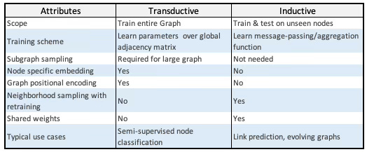
Table 1. Comparison of Transductive Graph Networks (e.g., GCN) and Inductive Graph Networks (e.g., GraphSAGE)
Graph Datasets
PyTorch Geometric (PyG) offers a comprehensive collection of graph datasets across various domains. These graph datasets are accessible through dedicated class in the torch_geometric.datasets module [ref 9]. There are more than 100 datasets, grouped into classes. Here are some examples:
Cora: A standard benchmark dataset for semi-supervised node classification, containing 2,708 nodes (scientific publications) and 5,429 edges (citations). Each node is described by a 1,433-dimensional feature vector. This dataset is also included in torch_geometric.datasets.Planetoid class collection.
CiteSeer: A citation network containing 3,312 scientific publications classified into six categories. The network contains 4,715 edges, with each node represented by a very large 3,703-dimensional feature vector. This dataset is also included in torch_geometric.datasets.Planetoid class collection.
PubMed: Consists of 19,717 scientific publications from the PubMed database, each pertaining to diabetes and classified into one of three classes. The citation network includes 44,338 edges, and each node has a 500-dimensional feature vector. This dataset is also included in torch_geometric.datasets.Planetoid class collection.
TUDatasets: This is a collection of graph dataset from TU Dortmund University which covers enzymes, proteins, and movies with an average of few thousand graphs and tens of nodes. It is defined in the torch_geometric.datasets.TUDatasets
Flickr: Contains descriptions and common properties of 89,250 images along with 899.756 edges and a 500-dimensional feature vector. It is defined in torch_geometric.datasets.Flickr class.
ZINC: A dataset from the ZINC database containing about 250,000 molecular graphs with up to 38 heavy atoms, used for molecular generation and property prediction tasks (torch_geometric.datasets..ZINC).
Yelp: dataset containing customer reviewers and their friendship with 716,847 nodes, 13,954,819 edges and a 300-dimensional feature vector (torch_geometric.datasets.Yelp).
KarateClub: This very small network contains 34 nodes, connected by 156 (undirected and unweighted) edges with a 34-dimensional feature vector (torch_geometric.datasets.KarateClub).
ShapeNet: A part-level segmentation dataset containing about 16,881 3D shape point clouds (graph) from 16 shape categories, 2,616 nodes (depending on sampling) and a 3-dimensional feature vector.
Reddit: A dataset containing Reddit posts belonging to different communities, with 232,965 nodes, 14,615,892 edges and a 602-dimensional feature vector, It is used for community detection and node classification tasks.
Amazon-Computer: Graph dataset with 3,752 nodes, 491,722 edges and a 767-dimensional feature vector. It is contained in the torch_geometric.datasets.Amazon dataset class.
Amazon-Photo: Graph dataset with 7,650 nodes, 238,162 edges and a 745-dimensional feature vector. It is contained in the torch_geometric.datasets.Amazon dataset class.
ModelNet40: Datasets containing 3D CAD designs with 12,311 graphs an average of 17,744 nodes and 66,060 edges (torch_geometric.datasets.ModelNet).
Graph Loaders
The generation of universal embeddings that apply across different applications remains a significant challenge.
PyTorch Geometric simplifies this process by encapsulating these complexities into specialized data loaders, while seamlessly integrating with PyTorch's existing deep learning modules.
The graph nodes and link loaders are an extension of PyTorch ubiquitous data loader. A node loader performs a mini-batch sampling from node information and a link loader performs a similar mini-batch sampling from link information.'
The latest version of PyTorch Geometric supports an extensive range of graph data loaders each associated with a specific layer sampling technique. Below is an illustration of the most commonly used node and link loaders. PyTorch Geometric supports a large variety of graph data loader, including:
Random node loader: A data loader that randomly samples nodes from a graph and returns their induced subgraph.
Neighbor node loader: This loader partitions nodes into batches and expands the subgraph by including neighboring nodes at each step. Each batch, representing an induced subgraph, starts with a root node and attaches a specified number of its neighbors.
Neighbor link loader: This loader is similar to the neighborhood node loader. It partitions links and associated nodes into batches and expands the subgraph by including neighboring nodes at each step.
Subgraphs Cluster: Divides a graph data object into multiple subgraphs or partitions. A batch is then formed by combining a specified number of subgraphs.
Graph Sampling Based Inductive Learning Method: This is an inductive learning approach that enhances training efficiency and accuracy by constructing mini-batches through sampling subgraphs from the training graph, rather than selecting individual nodes or edges from the entire graph.
⚙️ Hands-on with Python
The following implementation relies on the node neighborhood as layer sampling method, Graph Convolutional Network as model for the multi-label classification of Flickr images.
Environment
Libraries: Python 3.11.8, Numpy 1.26.4, PyTorch 2.1.0, PyTorch Geometric 2.6.1, torch-sparse: 0.6.18, torch-scatter: 2.1.2, torch-spline-conv: 1.2.2, torch-cluster: 1.6.3
Source code: geometriclearning/deeplearning/model/graph
To enhance the readability of the algorithm implementations, we have omitted non-essential code elements like error checking, comments, exceptions, validation of class and method arguments, scoping qualifiers, and import statements.
⚠️ Warning: Some sampling methods in PyTorch Geometric rely on additional modules: torch-sparse, torch-scatter, torch-spline-conv, and torch-cluster. These are dependencies of torch-geometric but they may not be compatible with the latest versions of PyTorch, particularly across different operating systems.
For macOS, we recommend the following version setup for best compatibility:
Python: 3.11.8
PyTorch: 2.1.0
torch-geometric: 2.6.1
torch-sparse: 0.6.18
torch-scatter: 2.1.2
torch-spline-conv: 1.2.2
torch-cluster: 1.6.3
These modules currently support only CPU and CUDA execution — MPS (Metal) is not supported.
🔎 Data Structure
The graph data is defined by the class torch_geometric.data.Data which has the following attributes:
data.x: Node feature matrix with shape [num_nodes, num_node_features]
data.edge_index: Graph connectivity with shape [2, num_edges] and type torch.long
data.edge_attr: Edge feature matrix shape [num_edges, num_edge_features]
data.y: Target to train against (may have arbitrary shape), e.g., node-level targets of shape [num_nodes, *] or graph-level targets of shape [1, *]
data.pos: Node position matrix with shape [num_nodes, num_dimensions].
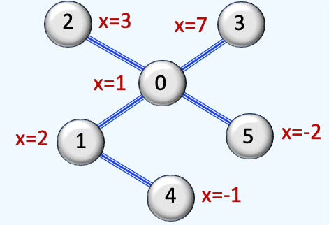
Let’s illustrate the attributes of the class Data with a simple 5 node graph:
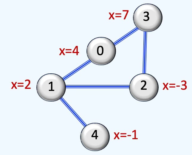
Fig. 2 Schema for a simple 5 node graph
The implementation consists of defining the node attribute data.x and the indices of nodes in the list of edges, edge_index.
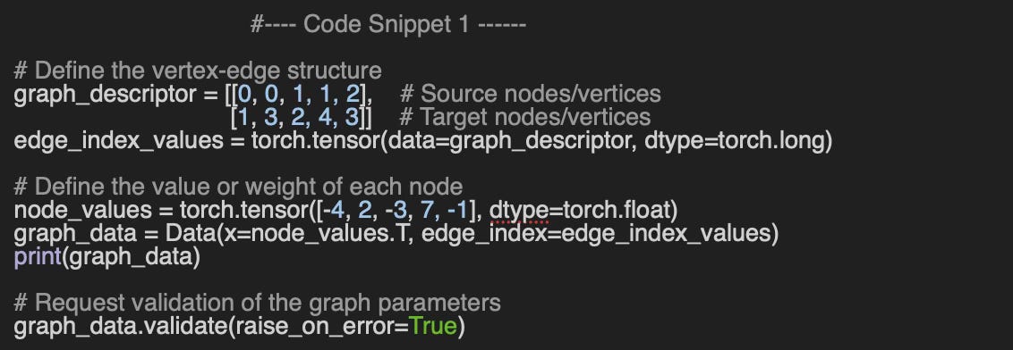
Data(x=[5], edge_index=[2, 5])🔎 Custom Loader
Let’s consider loading and visualizing the Flickr dataset with the neighbor node loader. The Flickr dataset is a graph where nodes represent images and edges signify similarities between them. It includes 89,250 images and 899,756 relationships. Node features consist of image descriptions and shared properties. This dataset is commonly used for tasks like node classification, link prediction, and graph representation learning.
📌 The Flickr dataset was previously utilized in a paper [ref 10] that employed a different layer sampling technique, known as Graph Sampling-Based Inductive Learning. In our Graph Neural Network (GNN) loader implementation, we opted for a simpler node neighborhood sampling strategy as an introduction to graph data loading techniques.
The neighbor node loader, described in the previous section, is implemented by the class from torch_geometric.loader.NeighborLoader which inherit from torch.utils.data.DataLoader and 3 other mixing classes.
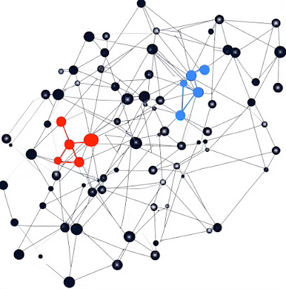
Fig. 3 Visualization of selection of graph nodes in a Neighbor node loader
The Flickr data set was used in a paper with a different layer sampling technique, Graph Sampling Based Inductive Learning method. We used the simpler node neighborhood sampling strategy in our initiation to Graph Neural Network loader.
⏭️ This section guides you through the design and code.
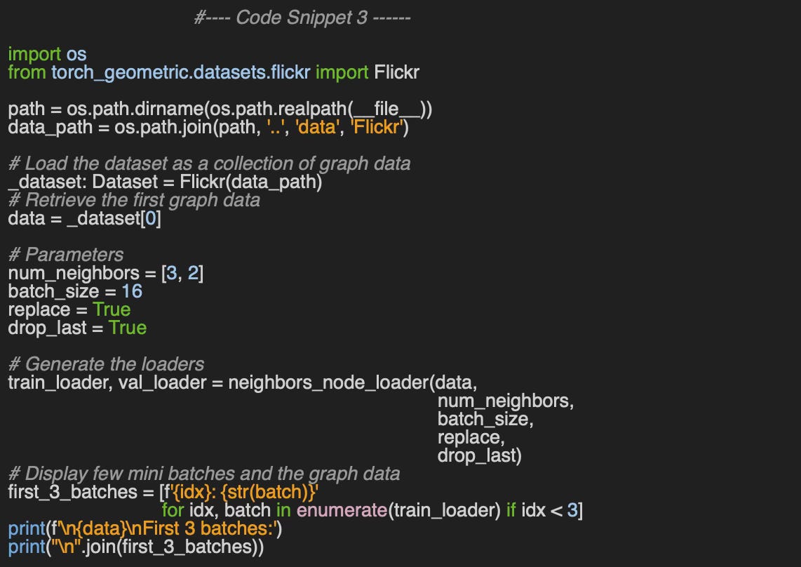
First we implement the function, neighbors_node_loader to generate the loader for the training and validation data. Beside the graph data, data, the loader relies on 4 configuration parameters:
num_neighbors: Number of neighbors used to sample each layer or hop of the Graph Neural Network. For instance, an input of [3, 2] directs the training to sample 3 nodes in the first hop (direct neighbors) and 2 nodes in the second hop.
batch_size: Defines the number of target nodes in each mini-batch used in training
replace: Specify if the sampling of neighbors is done with or without replacement.
drop_last_batch: Specify if the last batch if incomplete (Number of nodes is less than batch_size).
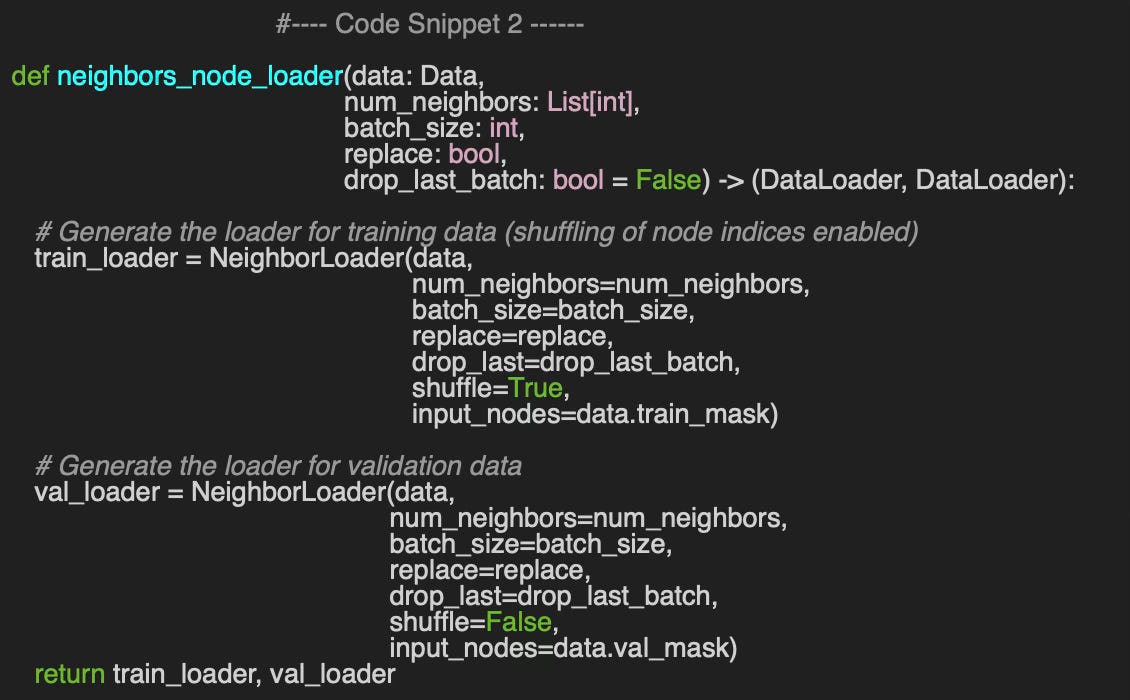
The training data loader shuffles the indices of input nodes, input_nodes specified by data.train_mask, whereas the validation loader does not.
For clarity, parallelism-related configuration parameters in training have been omitted.
Let’s extract the graph loaders for both training and validation data. In this example, the loader selects 3 nodes in the first hop and 2 nodes in the second hop for sampling with 16 nodes per mini-batch.
Output:
Data(x=[89250, 500], edge_index=[2, 899756], y=[89250],
     train_mask=[89250], val_mask=[89250], test_mask=[89250])
First 3 batches:
0: Data(x=[145, 500], edge_index=[2, 140], y=[145], train_mask=[145],
        val_mask=[145], test_mask=[145], n_id=[145], e_id=[140],
        input_id=[16], batch_size=16)
1: Data(x=[137, 500], edge_index=[2, 134], y=[137], train_mask=[137],
        val_mask=[137], test_mask=[137], n_id=[137], e_id=[134],
        input_id=[16], batch_size=16)
2: Data(x=[140, 500], edge_index=[2, 138], y=[140], train_mask=[140],
        val_mask=[140], test_mask=[140], n_id=[140], e_id=[138],
        input_id=[16], batch_size=16)
There are numerous libraries available for visualizing graphs, but over time, I have found NetworkX [ref 11, 12] to be one of the most expressive. A comprehensive overview of NetworkX's capabilities will be covered in a future article.
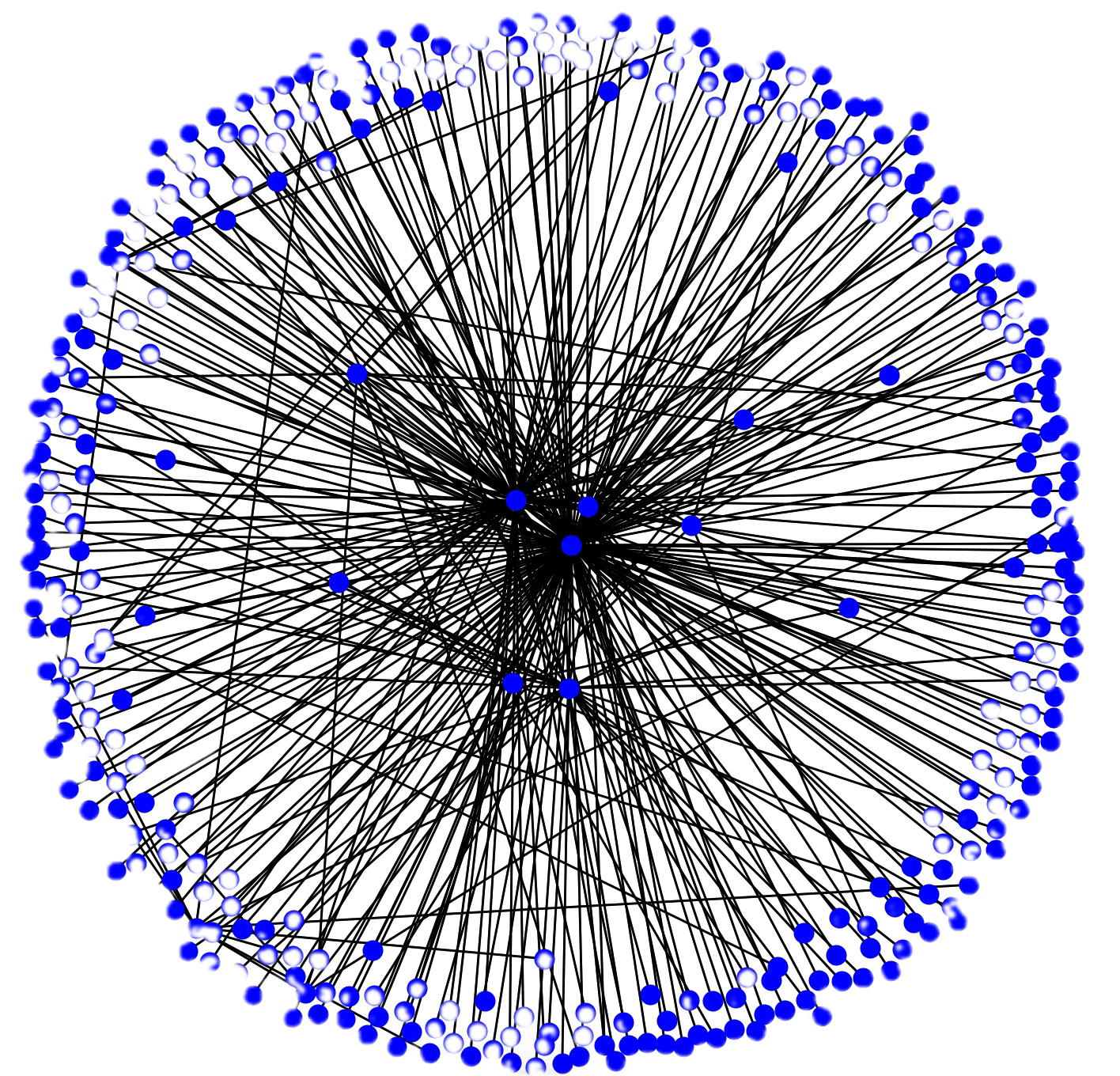
Fig. 4 Display of sampled sub-graph from Flickr data set using NetworkX spring layout
Graph Neural Model
Graph Neural Networks can be quite intricate, so we use reusable building blocks to streamline the structure of various PyTorch modules. Detailed information regarding reusable neural blocks is available in this newsletter at Reusable Neural Blocks in PyTorch
PyTorch Geometric provides numerous configuration options for building a Graph Neural Network, which can sometimes feel overwhelming. To illustrate the challenges data scientists and engineers face in designing and fine-tuning the best model for their graph dataset, we focus on the widely used Graph Convolutional Network.
Graph Convolutional Neural Block
The first step is to define the logical grouping of all possible PyTorch module associated with a graph convolutional layer required for training:
Message-passing layer or Convolutional layer
Batch normalization
Activation function
Pooling module
Optional dropout regularization for training
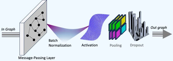
Fig. 5 Illustration of the components of a Graph Convolutional Neural Block
To achieve this, we define a Graph Convolutional Network block, GraphConvBlock, which encapsulates the essential neural components required to train a single layer with the following transformer X → X’using the Adjacency matrix A and degree matrix D.
🔎 The components of a Graph Convolutional block is defined by the following module
graph_conv_layer: Graph convolutional operator which type is either GraphConv, GCNConv or GCN2Conv.
batch_norm: Optional module that applies batch normalization over a batch of features
activation_module: Optional activation function associated with the convolutional operator
pooling_module: Optional hierarchical pooling module for node-level classification of type either TopKPooling or SAGPooling.
drop_out_module: Optional PyTorch module for dropout weights regularization used in training.
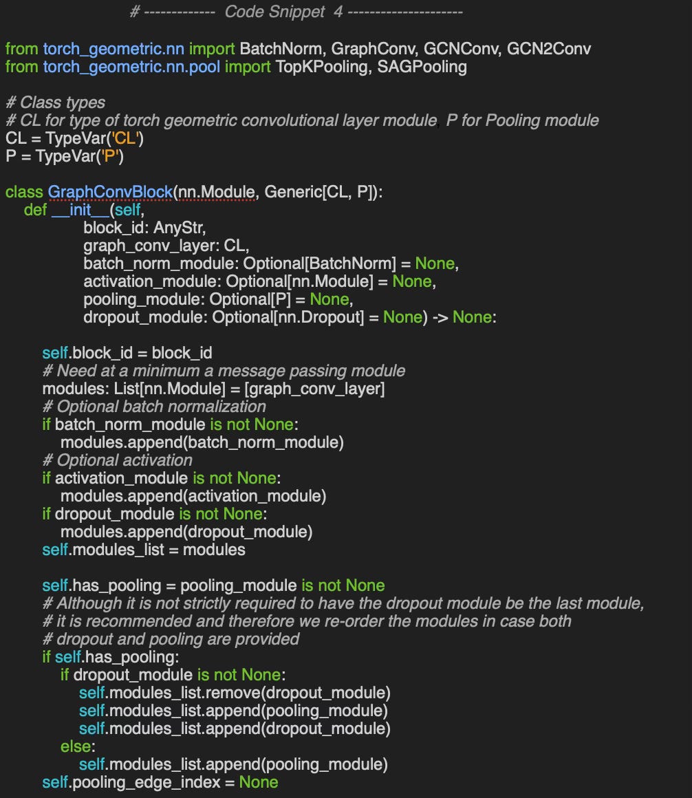
The constructor raises a TypeError exception if the convolutional module, graph_conv_layer is not of type GraphConv, GCNConv or GCN2Conv or pooling module, pooling_module is not of type TopKPooling or SAGPooling. The validation code is not shown for sake of clarity.
The constructor dynamically assembles the sequence of Torch modules in the order specified by the arguments.
📌 Although not strictly required we make sure that the dropout module is the last module.
The forward method for the block is described in the Code snippet 5.
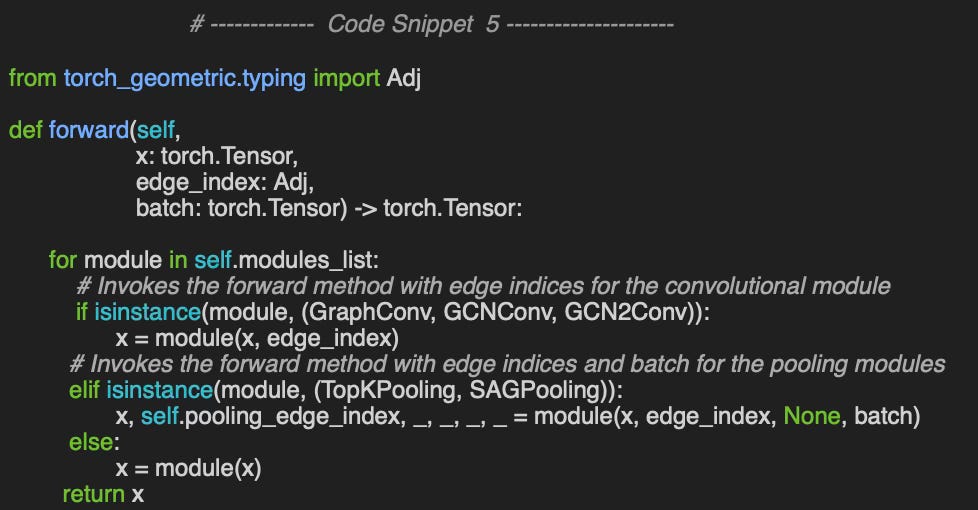
Configurability Challenges
The GraphConvBlock supports two types of graph convolutional operators - GraphConv, GCNConv or GCN2Conv —along with two pooling strategies: TopKPooling and SAGPooling . The challenge lies in selecting the right combination of parameters best suited for the dataset.
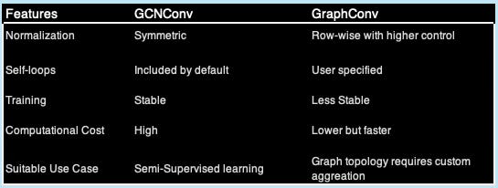
GraphConv vs. GCNConv
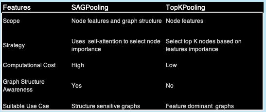
SAGPooling vs. TopKPooling
The purpose of the pooling module is to reduce the number of nodes in a graph while retaining important information, making them useful for graph classification and large-scale graph learning. Although Both TopKPooling and SAGPooling are hierarchical pooling techniques, there are some notable differences:
Graph Convolutional Network
A General Graph Convolutional Network is composed of a sequence of graph convolutional blocks, fully connected feedforward layers, and a Softmax activation function for classification, as illustrated below.
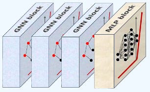
Fig. 6 A 3-layer graph convolutional neural network for Flickr data set
🔎 Let's define a class, GraphConvModel. to implement our Graph Convolutional Network (GCN), structured as a sequence of Graph Convolutional Blocks (type GraphConvBlock), stored in gconv_blocks, along with a set of fully connected perceptron blocks (type MLPBlock) stored in mlp_blocks.
The class GraphConvModel inherits torch Module so the model can implicitly invokes its forward method.
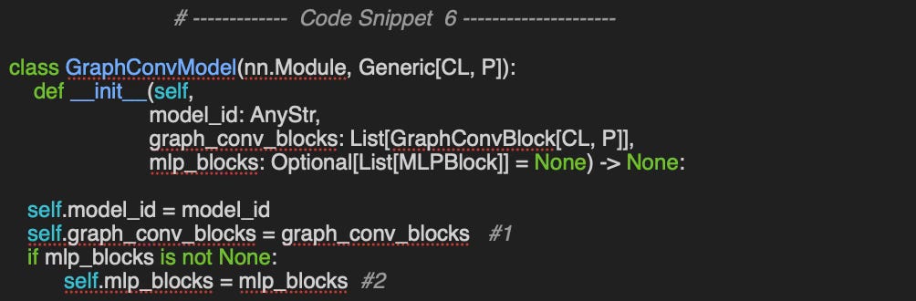
The constructor extracts the torch modules from the convolutional neural blocks (#1) and fully connected blocks (#2) if specified.
The forward method invokes iteratively its namesake for the graph convolution blocks, and if needed, for the multi-layer perceptron blocks.
Recursive hierarchical forward invocation
Neural blocks are designed to encapsulate a set of PyTorch modules, each performing a specific function. As a result, when the __call__ method is implicitly invoked on a model such as GraphConvModel, it triggers the forward method of each neural block. In turn, each neural block sequentially executes the forward method of all the PyTorch modules it contains.
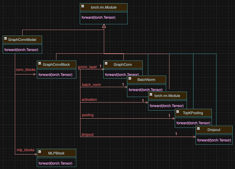
Fig. 7 Class diagram for GraphConvModel and its Neural Blocks
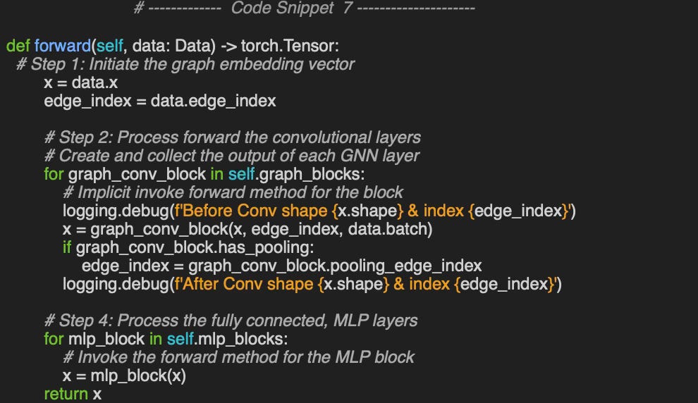
🔎 The forward method follows four key steps:
Initialize the graph embedding vector.
Pass input data through the Graph Convolutional Neural Blocks using the corresponding PyTorch modules.
Flatten the output from the final convolutional block by applying concatenation.
Process the flattened data through the fully connected (MLP) blocks using their associated PyTorch modules.
Finally, let’s build the model to classify Flickr images with 2 fully equipped graph convolutional blocks (batch normalization, activation function, pooling and dropout), 1 convolutional layer block and 1 fully connected output layer with a Softmax activation.

Output:
0: GraphConv(500, 256)
1: BatchNorm(256, eps=1e-05, momentum=0.1, affine=True,
             track_running_stats=True)
2: ReLU()
3: TopKPooling(256, ratio=0.4, multiplier=1.0)
4: Dropout(p=0.2, inplace=False)
5: GraphConv(256, 256)
6: BatchNorm(256, eps=1e-05, momentum=0.1, affine=True,
             track_running_stats=True)
7: ReLU()
8: TopKPooling(256, ratio=0.4, multiplier=1.0)
9: Dropout(p=0.2, inplace=False)
10: GraphConv(256, 256)
11: Flatten(start_dim=1, end_dim=-1)
12: Linear(in_features=256, out_features=7, bias=True)
13: Softmax(dim=-1)
🧠 Takeways
✅ PyTorch Geometric is a powerful and extensive library for implementing Graph Neural Networks (GNNs), though its complexity can be overwhelming for beginners.
✅ Designing GNN models involves making key trade-offs in choosing the right models, samplers, and data loaders.
✅ NetworkX is Python graphical library with great support for representing large graphs.
✅ Using reusable neural blocks provides an efficient way to structure PyTorch modules, enabling the creation of complex neural networks with better modularity and organization.
📘 References
Fast Graph Representation Learning with PyTorch Geometric M. Fey, J. Lenssen - Dept. Computer Graphics - TU Dortmund University
PyTorch Geometric Documentation pyg.org
A Practical Tutorial on Graph Neural Networks I. Ward, J. Joyner, C. Lickfold, Y. Guo, M. Bennamoun
YouTube: Build your first GNN A. Nandakumar
YouTube: Graph Representation Learning - Stanford Education class CS224w-2018
YouTube: ntroduction to Graph Neural Networks - P. Veličković
Foundations and Frontiers of Graph Learning Theory Y. Huang et all. - IEEE
Theory of Graph Neural Networks: Representation and Learning. S. Jegelka - CSAIL, MIT
GraphSAINT: Graph Sampling Based Inductive Learning Method H.Zeng, H. Zhou, A. Srivastava, R. Kannan, V. Prasanna
Visualization of Graph Neural Networks P Nicolas
🛠️ Q&A
Q1: What does edge_index represent in the context of graph data (type Data)?
Q2: How can you create a Data instance for the given graph using PyTorch Geometric?
Q3: What is the role of data.train_mask in graph-based learning?
Q4: Between GraphConv and GCNConv, which Graph Convolutional operator offers greater stability?
👉 Answers
💬 News & Reviews
This section focuses on news and reviews of papers pertaining to geometric deep learning and its related disciplines.
Paper review: Manifold Matching via Deep Metric Learning for Generative Modeling M. Day, H. Hang
Overview
This study advances the recent progress in blending geometry with statistics to enhance generative models. It proposes a novel method for identifying manifolds within Euclidean spaces for generative models like variational encoders and GANs through two neural networks:
Data generator sampling data on the manifold
Metric generator learning geodesic distances.
Metric learning
The metric generator produces a pullback of the Euclidean space while the data generator produces a push forward of the prior distribution. The algorithm is described with easy-to-follow pseudo code.
The method is tested on unconditional ResNet image creation and GAN-based image super-resolution, showing improved Frechet Inception Distance and Perception Scores.
This paper will be especially of interest to engineers already familiar with GANs and Frechet metric.
Expertise Level
⭐ Beginner: Getting started - no knowledge of the topic
⭐⭐ Novice: Foundational concepts - basic familiarity with the topic
⭐⭐⭐ Intermediate: Hands-on understanding - Prior exposure, ready to dive into core methods
⭐⭐⭐⭐ Advanced: Applied expertise - Research oriented, theoretical and deep application
⭐⭐⭐⭐⭐ Expert: Research , thought-leader level - formal proofs and cutting-edge methods.
Share the next topic you’d like me to tackle.
Patrick Nicolas is a software and data engineering veteran with 30 years of experience in architecture, machine learning, and a focus on geometric learning. He writes and consults on Geometric Deep Learning, drawing on prior roles in both hands-on development and technical leadership. He is the author of Scala for Machine Learning (Packt, ISBN 978-1-78712-238-3) and the newsletter Geometric Learning in Python on LinkedIn.