

Demystifying Graph Sampling & Walk Methods
Expertise Level ⭐⭐⭐

The versatility of graph representations makes them highly valuable for solving a wide range of problems, each with its own unique data structure. However, generating universal embeddings that apply across different applications remains a significant challenge.
This article explores PyTorch Geometric (PyG) data loaders and presents a streamlined interface to abstract away their underlying complexity.

🎯 Why this Matters
Purpose: The wide range of datasets and samplers available in PyTorch Geometric can be overwhelming at first. To simplify exploration, we’ve developed interfaces that make it easier to navigate and experiment with different datasets and sampling strategies.
Audience: Data scientists leveraging the vast array of PyTorch Geometric functionality to build Graph Neural Networks
Value: Learn how graph data loaders influence node classification in a Graph Neural Network implemented with PyTorch Geometric and leverage easy-to-use interfaces o kickstart your exploration of the various architectures.
⚠️ Warning: Some sampling methods in PyTorch Geometric rely on additional modules: torch-sparse, torch-scatter, torch-spline-conv, and torch-cluster. These are dependencies of torch-geometric but they may not be compatible with the latest versions of PyTorch, particularly across different operating systems.
For macOS, we recommend the following version setup for best compatibility:
Python: 3.11.8
PyTorch: 2.1.0
torch-geometric: 2.6.1
torch-sparse: 0.6.18
torch-scatter: 2.1.2
torch-spline-conv: 1.2.2
torch-cluster: 1.6.3
These modules currently support only CPU and CUDA execution — MPS (Metal) is not supported.
🎨 Modeling & Design Principles
Overview
Data on manifolds can often be represented as a graph, where the manifold's local structure is approximated by connections between nearby points. GNNs and their variants (like Graph Convolutional Networks (GCNs)) extend neural networks to process data on non-Euclidean domains by leveraging the graph structure, which may approximate the underlying manifold. Application Social network analysis, molecular structure prediction, and 3D point cloud data can all be modeled using GNNs.
I strongly recommend to review my article introducing PyTorch Geometric Taming PyTorch Geometric for Graph Neural Networks
📌 The description of the inner-workings and mathematical foundation of graph neural networks, message passing architecture and aggregation policies are beyond the scope of this article. Some of the most relevant tutorials and presentations on GNNs are listed in references [ref 2, 3, 4 & 5].
Graph Neural Networks
The variety of Graph Neural Network (GNN) architectures has grown rapidly over the past three years, driven by a surge in technical publications on the subject.
Here’s a shortlist of some of the most widely used GNN models.
Graph Convolutional Networks (GCNs): GCNs generalize the concept of convolution from grids (e.g., images) to graphs. They aggregate information from a node's neighbors using normalized adjacency matrices and apply transformations to learn node embeddings.
Graph Attention Networks (GATs): GATs use attention mechanisms to learn the importance of neighboring nodes dynamically. Each edge is assigned a learned weight during aggregation.
GraphSAGE (Graph Sample and Aggregate): It learns node embeddings by sampling and aggregating features from a fixed-size neighborhood of each node, enabling scalable learning on large graphs.
Graph Isomorphism Networks (GINs): GINs are designed to be as powerful as the Weisfeiler-Lehman (WL) graph isomorphism test, distinguishing graph structures more effectively.
Spectral Graph Neural Networks (SGNN): These networks operate in the spectral domain using the graph Laplacian. They use eigenvectors of the Laplacian for convolution-like operations.
Graph Pooling Networks: They summarize graph information into a smaller representation, similar to pooling in CNNs. They can be categorized into Global and hierarchical pooling
Hyperbolic Graph Neural Networks: These networks operate in hyperbolic space, which is well-suited for representing hierarchical or tree-like graph structures.
Dynamic Graph Neural Networks: These networks are designed to handle temporal graphs, where nodes and edges evolve over time.
Relational Graph Convolutional Networks (R-GCNs): R-GCNs extend GCNs to handle heterogeneous graphs with different types of nodes and edges.
Graph Transformers: They adapt the Transformer architecture to graph-structured data using attention mechanisms and global context.
Graph Autoencoders: These are used for unsupervised learning on graphs, aiming to reconstruct graph structure and node features.
Diffusion-Based GNNs: These networks use graph diffusion processes to propagate information.
PyTorch Geometric
PyTorch Geometric (PyG) is a graph deep learning library built on PyTorch, designed for efficient processing of graph-structured data. It provides essential tools for building, training, and deploying Graph Neural Networks (GNNs) [ref 6].
The key Features of PyG are:
Efficient Graph Processing to optimize memory and computation using sparse graph representations.
Flexible GNN Layers that includes GCN, GAT, GraphSAGE, GIN, and other advanced architectures.
Batching for Large Graphs to support mini-batching for handling graphs with millions of edges.
Seamless PyTorch Integration with full compatibility with PyTorch tensors, autograd, and neural network modules.
Diverse Graph Support for directed, undirected, weighted, and heterogeneous graphs.
The most important PyG Modules are:
torch_geometric.data to manages graph structures, including nodes, edges, and features.
torch_geometric.nn to provide data scientists prebuilt GNN layers like convolutional and gated layers.
torch_geometric.transforms to pre-process input data (e.g., feature normalization, graph sampling).
torch_geometric.loader to handle large-scale graph datasets with specialized loaders.
Graph Samplers
Overview
Some real-world applications involve handling extremely large graphs with thousands of nodes and millions of edges, posing significant challenges for both machine learning algorithms and visualization. Fortunately, PyG (PyTorch Geometric) enables data scientists to batch nodes or edges, effectively reducing computational overhead for training and inference in graph-based models.
First we need to introduce the attributes of the data of type torch_geometric.data.Data that underline the representation of a graph in PyG.
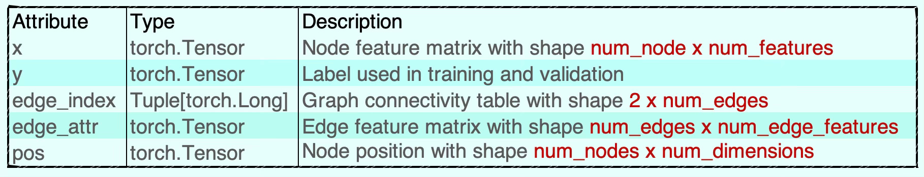
Table 1. Attributes of graph data in PyTorch Geometric
Data Splits
The graph is divided into training, validation, and test datasets by assigning train_mask, val_mask, and test_mask attributes to the original Data object, as demonstrated in the following code snippet.
# 1. Define the indices for training, validation and test data points
train_idx = torch.tensor([0, 1, 2, 4, 6, 7, 8, 11, 12, 13, 14])
val_idx = torch.tensor([3, 9, 14])
test_idx = torch.tensor([5, 10])

#2. Verify all indices are accounted for with no overlap
validate_split(train_idx, val_idx, test_idx)

#3. Get the training, validation and test data set
train_data = data.x[train_idx], data.y[train_idx]
val_data = data.x[val_idx], data.y[val_idx]
test_data = data.x[test_idx], data.y[test_idx]
Alternatively, we can use the RandomNodeSplit and RandomLinkSplit classes to directly extract the training, validation, and test datasets.
from torch_geometric.transforms import RandomNodeSplit

transform = RandomNodeSplit(is_undirected=True)
train_data, val_data, test_data = transform(data)
Common Sampling Architectures
The graph nodes and link samplers are an extension of PyTorch ubiquitous data loader. A node loader performs a mini-batch sampling from node information and a link loader performs a similar mini-batch sampling from link information.'
The latest version of PyG supports an extensive range of graph data loaders. Below is an illustration of the most commonly used node and link loaders.
📌 As PyG implements node and edge sampling methods through data set loaders in PyG, we use the terms sampler and loader interchangeably.
Random Node Sampling
A data loader that randomly samples nodes from a graph and returns their induced subgraph. In this case, the two sampled subgraphs are highlighted in blue and red.
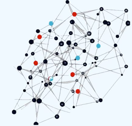
Fig 1. Visualization of selection of graph nodes in a Random node loader
Neighbor Node Sampling
This loader partitions nodes into batches and expands the subgraph by including neighboring nodes at each step. Each batch, representing an induced subgraph, starts with a root node and attaches a specified number of its neighbors. This approach is similar to breath-first search in trees.

Fig 2. Visualization of selection of graph nodes in a Neighbor node loader
Neighbor Link Sampling
This loader is similar to the neighborhood node loader. It partitions links and associated nodes into batches and expands the subgraph by including neighboring nodes at each step.
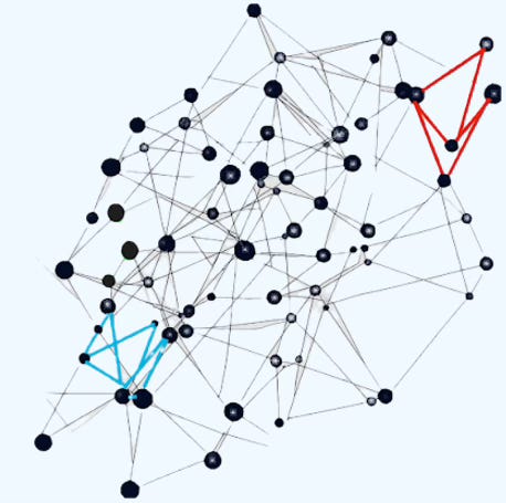
Fig 3. Visualization of selection of graph nodes in a Neighbor link loader
Subgraphs Cluster Sampling
Divides a graph data object into multiple subgraphs or partitions. A batch is then formed by combining a specified number (`batch_size`) of subgraphs. In this example, two subgraphs, each containing five green nodes, are grouped into a single batch.
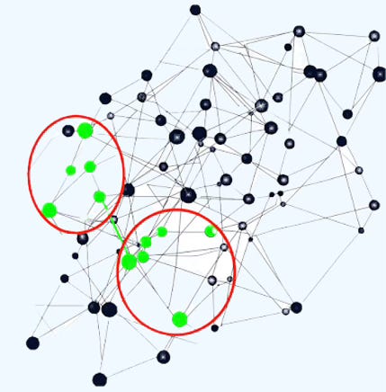
Fig 4. Visualization of selection of graph nodes in a cluster loader
Graph Sampling Based Inductive Learning Method
This is an inductive learning approach that enhances training efficiency and accuracy by constructing mini-batches through sampling subgraphs from the training graph, rather than selecting individual nodes or edges from the entire graph. This approach is similar to depth-first search in trees.
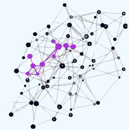
Fig 5. Visualization of selection of graph nodes in a Graph SAINT random walk
⚙️ Hands-on with Python
Environment
Libraries: Python 3.11.8, PyTorch 2.1.0, PyTorch Geometric 2.6.1, torch-sparse: 0.6.18, torch-scatter: 2.1.2, torch-spline-conv: 1.2.2, torch-cluster: 1.6.3
Source code: geometriclearning/dataset/graph/graph_data_loader.py
Evaluation code :geometriclearning/play/graph_data_loader_play.py
The source tree is organized as follows: features in python/, unit tests in tests/,and newsletter evaluation code in play/.
To enhance the readability of the algorithm implementations, we have omitted non-essential code elements like error checking, comments, exceptions, validation of class and method arguments, scoping qualifiers, and import statements.
⚠️This article explores the PyG (PyTorch Geometric) Python library to evaluate various graph neural network (GNN) architectures. It is not intended as an introduction or overview of GNNs and assumes the reader has some prior knowledge of the subject.
🔎 Datasets
The PyTorch Geometric library offers a wide range of datasets that data scientists can use to evaluate different Graph Neural Network architectures [ref 7].
Since each dataset may follow its own loading and extraction protocol, we'll create a convenient wrapper class called, PyGDatasets to serve as a unified interface—abstracting away the underlying implementation details.
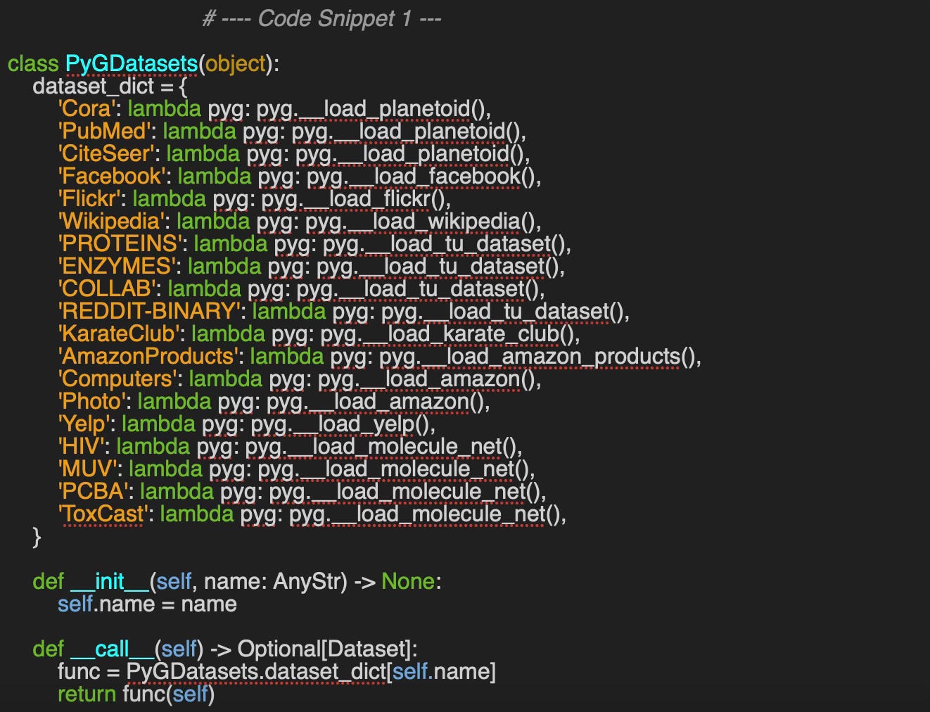
Here is an example of a private loading method:
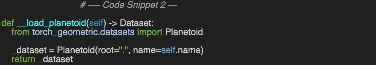
The data for each source can be simply extracted as:

CiteSeer:
Data(x=[3327, 3703], edge_index=[2, 9104], y=[3327], train_mask=[3327], val_mask=[3327], test_mask=[3327])
🔎 Graph Data Loader
⏭️ This section guides you through the design and code—skip if you only want results.
Let's analyze the impact of different graph data loaders on the performance of a Graph Convolutional Neural Network (GCN).
To facilitate this evaluation, we'll create a wrapper class, GraphDataLoader, for managing the access and loading of graph data.
As shown in code snippet #4, we've organized the different loading and sampling methods into a dictionary called loader_sampler_dict, where each sampler name serves as a key and the corresponding data loading lambda function is the value.
The arguments of the constructor are:
loader_attributes: Dictionary for the configuration of this specific loader
dataset_name: Name of the PyG dataset
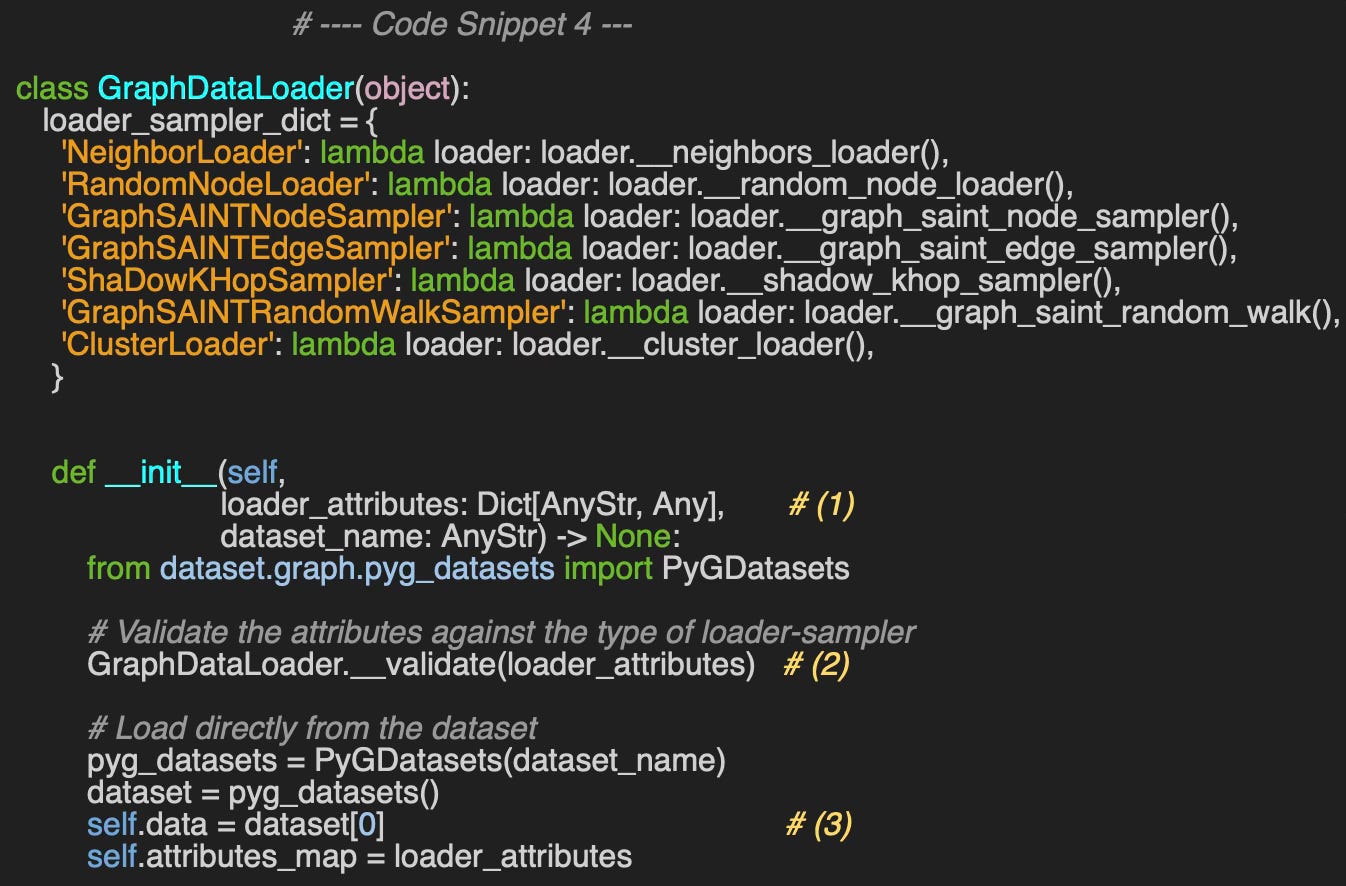
The dictionary of the attributes (1) is specific to the loader and therefore needs to be validated (2). For instance the attributes for accessing Flickr dataset using neighbor loader is defined as
loader_attributes={
   'id': 'NeighborLoader',
   'num_neighbors': [3, 2],
   'batch_size': 4,
   'replace': True,
   'num_workers': 1}
The data is extracted as the first entry in the dataset (3).
The __call__ method directs requests to the appropriate node or link loader-sampler.

To keep this article concise, our evaluation focuses on the following three graph data loaders:
Random Nodes
Neighbors Nodes
Graph SAINT Random Walk
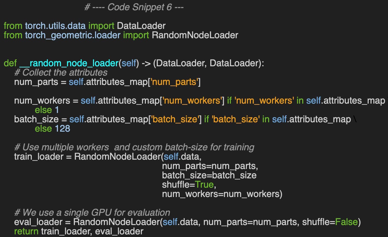
Random Node Loader
The only configuration 3 attributes for the random node loader are
num_parts: Number of subgraphs generated through partitioning and sampling of the input graph. The data set is split into num_parts subgraphs to improve performance and parallelization for large graphs.
batch_size: Number of graph nodes used in a mini-batch
num_workers: Number of concurrent execution for training and validation.
📌 The meaning of batch_size varies depending on the type of graph task: for graph-level tasks (e.g., graph classification), it refers to the number of graphs per mini-batch; for node-level tasks, it’s the number of nodes per mini-batch; and for edge-level tasks, it represents the number of edges per mini-batch.
The loader for the training set shuffles the data while the order of data points for the validation set is preserved.
We consider the Flickr data set included in PyTorch Geometric. The Flickr dataset is a graph where nodes represent images and edges signify similarities between them [ref 8]. It includes 89,250 images and 899,756 relationships. Node features consist of image descriptions and shared properties.
The purpose is to classify Flickr images (defined as graph nodes) into one of the 108 categories.
👉 Source code is available at geometriclearning/play/graph_data_loader_play.py
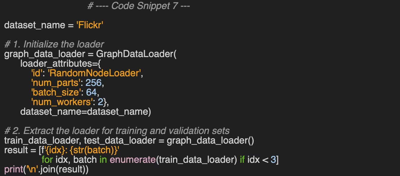
0: Data(x=[349, 500], edge_index=[2, 8], y=[349], train_mask=[349], val_mask=[349], test_mask=[349])
1: Data(x=[349, 500], edge_index=[2, 12], y=[349], train_mask=[349], val_mask=[349], test_mask=[349])
2: Data(x=[349, 500], edge_index=[2, 6], y=[349], train_mask=[349], val_mask=[349], test_mask=[349])
We train a three-layer Graph Convolutional Neural Network (GCN) on the Flickr dataset for classify these images into 108 categories. In this first experiment the model trains on data extracted by the random node loader. For clarity, the code for training the model, computing losses, and evaluating performance metrics has been omitted.
📌 The training and evaluation of Graph Neural Networks is outside the scope of this article and will be covered in future installments.
The following plot tracks the various performance metrics (accuracy, precision and recall) as well as the training and validation loss over 60 iterations.
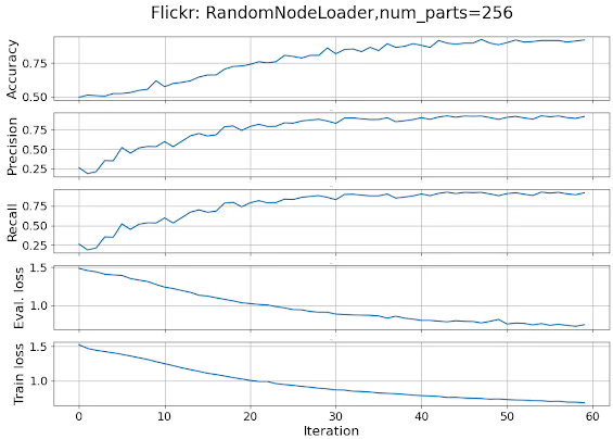
Fig 6. Performance metrics and loss for a GCN in a multi-label classification of data loaded randomly
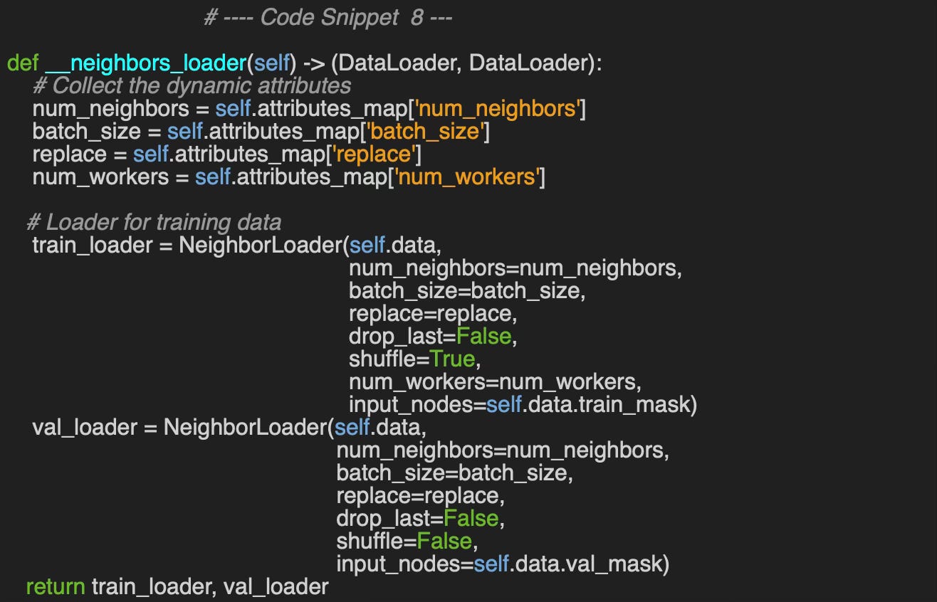
🔎 Neighbor Node Loader
The configuration parameters used for this loader include:
num_neighbors: Number of neighbors to sample at each layer or hop in a Graph Neural Network. It is defined as an array, e.g., [num_neighbors_first_hop, num_neighbors_second_hop, ...].
replace: Flag that specifies if a sampling is performed with or without replacement.
batch_size: Number of graph nodes in a min_batch.
num_workers: Number of concurrent executions for training and validation
We specify few other parameters which value do not vary during our evaluation>
drop_last: Flat that specifies whether the last min-batch has to be dropped if its size < batch_size
input_nodes Target graph nodes (training or validation) using data split and mask.
📌 Increasing the number of hops when sampling neighboring nodes helps capture long-range dependencies, but it comes with increased computational cost. Moreover, for most tasks, performance tends to degrade beyond three hops. Regardless of the depth, the number of sampled nodes in the first hop should be larger than in the second hop, and this pattern should continue for subsequent hops
Running the code described in snippet 7, with the attributes
{
  'id': 'NeighborLoader',
  'num_neighbors': [6, 2],
  'replace': True,
  'batch_size': 1024,
  'num_workers': 4
}
produces the following plots for the performance metrics and losses.
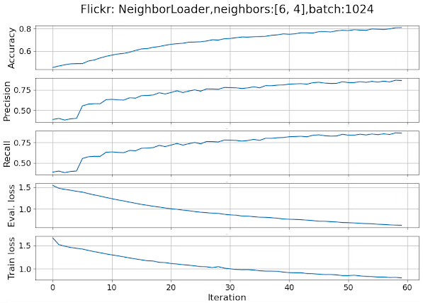
Fig 7. Performance metrics and loss for a GCN in a multi-label classification of data loaded with a Neighbor loader
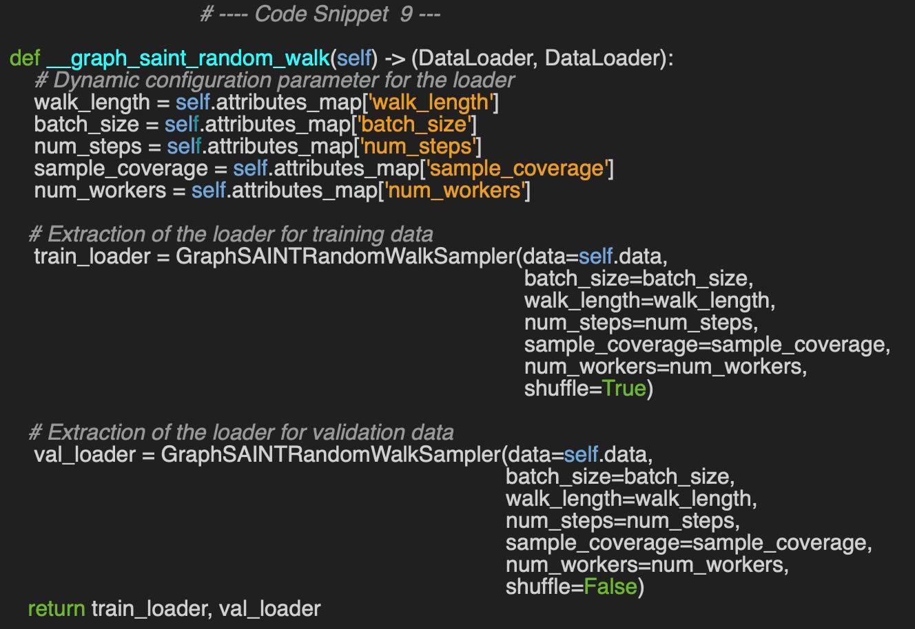
🔎 Graph Sampling Based Inductive Learning Loader
For evaluating this loader, we use the following configuration parameters:
walk_length: Number of hops (nodes) in a single random walk
batch_size: Size of the batch of graph nodes
num_steps: Number of times new nodes are samples in each epoch
sample_coverage: Number of times each node is sampled as appeared in a min-batch.
num_workers: Number of concurrent execution for training and validation
Running the code described in snippet 7, with the attributes
{
  'id': 'GraphSAINTRandomWalkSampler',
  'walk_length':3,
  'num_steps': 12,
  'sample_coverage': 100,
  'batch_size': 4096,
  'num_workers': 4
}
produces the following plots for the performance metrics and losses.
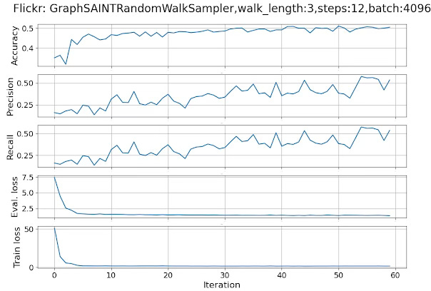
Fig 8. Performance metrics and loss for a GCN in a multi-label classification of data loaded with a Graph SAINT random walk loader
The performance metrics, accuracy, precision and recall points to an inability for the Random walk to capture long-range dependencies.
Comparative Analysis
Lastly, let's compare the impact of each data loader-sampler on the precision of the graph convolutional neural network.
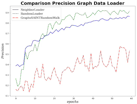
Fig 9. Plotting precision in a multi-label classification of a GCN with various graph data loaders
Although the random walk for the GraphSAINTRandomWalk loader excels in analyzing and representing local structure, it fails to capture the global context (high number of hops - dependencies) of a large image set. Moreover, the plot highlights the high degree of instability of performance metrics even though the loss in the validation run converges appropriately.
NeighborNodeLoader select nodes across multiple hops and therefore avoid over emphasis on nodes sampled in nearby regions
🧠 Key Takeaways
✅ We defined a single, user-friendly interface to access the wide selection of datasets and sampling strategies offered in PyTorch Geometric
✅ Creating a sampler-loader from a dictionary of attributes streamlines the process of building and evaluating Graph Neural Network models.
✅ Graph nodes and edges can be sampled using random or deterministic walks, each with its own trade-offs as discussed in the research literature.
✅ Each loader-node sampler have unique applicability criteria and limitations

📘 References
Taming PyTorch Geometric for Graph Neural Networks P. Nicolas - 2025
A Practical Tutorial on Graph Neural Networks I. Ward, J. Joyner, C. Lickfold, Y. Guo, M. Bennamoun - 2012
A Comprehensive Introduction to Graph Neural Networks - Datacamp - 2022
Graph Neural Networks: A Gentil Introduction - YouTube. A. Persson
Stanford CS: Machine Learning with Graphs - YouTube - CS-224 Stanford University Online
🛠️ Q&A
Q1. Is a graph sampling-based inductive learning method conceptually similar to:
Breadth-first search (BFS)? Depth-first search (DFS)?
Q2. In the context of edge prediction on a graph, what does batch_size represent?
Q3. How can you differentiate between training and validation data when using a neighbor sampling loader?
Q4. Which of the following num_neighbors configurations is most suitable for a neighbor sampler: [4, 8, 8], [8, 4, 2], [8, 4, 4, 2]?
Q5. Can you provide a code snippet to create a neighbor sampling loader for the Facebook dataset using PyTorch, following the structure of Code Snippet #2?
👉 Answers
💬 News & Reviews
This section focuses on news and reviews of papers pertaining to geometric deep learning and its related disciplines.
Paper review: Variational Transformer Autoencoder with Manifolds Learning P. Shamsolmoali, M. Zareapoor, H. Zhou, D. Tao - IEEE
The paper illustrates how the Riemann metric effectively addresses the challenges of modeling non-linear latent spaces by interpolating between input data samples along geodesics. The researchers have developed a variational autoencoder that incorporates a spatial transformer as the encoder to map the latent space model onto a Riemann manifold.
The goal is to refine the variational auto-encoder to calculate the geodesic distances between input data points, utilizing the Riemann metric tensor, and to delineate a semantic feature/latent space. The encoded transformer component is responsible for calculating the prior in the latent space. Importantly, this new model does not necessitate any modifications to the existing loss function (ELBO) or the training methodology.
Implemented in PyTorch, the model consists of four convolutional layers, two linear reshaping layers, and fifty latent variables. It has been evaluated using a variety of image sets, including grayscale images (such as MNIST and FashionMNIST) and color, natural images (such as CelebA and CIFAR-10). The proposed model demonstrates substantial improvements in image reconstruction.
Note: The paper assumes knowledge of differential geometry and generative models. The source code is available on GitHub.
Expertise Level
⭐ Beginner: Getting started - no knowledge of the topic
⭐⭐ Novice: Foundational concepts - basic familiarity with the topic
⭐⭐⭐ Intermediate: Hands-on understanding - Prior exposure, ready to dive into core methods
⭐⭐⭐⭐ Advanced: Applied expertise - Research oriented, theoretical and deep application
⭐⭐⭐⭐⭐ Expert: Research , thought-leader level - formal proofs and cutting-edge methods.
Share the next topic you’d like me to tackle.
Patrick Nicolas is a software and data engineering veteran with 30 years of experience in architecture, machine learning, and a focus on geometric learning. He writes and consults on Geometric Deep Learning, drawing on prior roles in both hands-on development and technical leadership. He is the author of Scala for Machine Learning (Packt, ISBN 978-1-78712-238-3) and the newsletter Geometric Learning in Python on LinkedIn.