

Geometry of Closed-Form Statistical Manifolds
Expertise Level ⭐⭐

Machine learning models grounded in information geometry can be challenging due to the intractability of their geometric properties.
This article, the first in a series dedicated to information geometry, explores simpler, closed-form statistical manifolds that offer practical insights for developing geometry-aware deep learning models.

🎯 Why this matters
Purpose: Statistical manifolds generalize the concept of Riemannian manifolds to the space of probability distributions. While their geometric properties—such as exponential and logarithm maps or distance—are often intractable, univariate distributions typically allow for closed-form or analytical expressions of these properties.
Audience: Data scientists and engineers involved in model relying on information geometry.
Value: Discover how to easily compute the geometric properties of closed-form statistical manifolds, including the Exponential, Binomial, and Geometric distributions.
🎨 Modeling & Design Principles
📌 This article explores key components of Fisher-Riemannian manifolds, including geodesics, as well as the exponential and logarithmic maps. A subsequent article will delve into applying the Fisher-Rao information metric to compute geodesic distances and inner products.
Overview
Information geometry is a branch of mathematics that leverages differential geometry to analyze the structure of statistical models. Its central idea is to treat families of probability distributions as geometric objects called statistical manifolds.
A statistical manifold is a smooth manifold in which each point represents a probability distribution, parameterized by one or more variables—for example, the rate parameter in an exponential distribution or the mean and standard deviation in a normal distribution.
By extending Riemannian geometry to the space of probability density functions, statistical manifolds provide a geometric framework for statistical inference. As such, a foundational understanding of differential geometry and Riemannian manifolds is recommended for readers.
Information geometry has various applications to machine learning:
Bayesian inference using divergence (Kullback-Leibler, Bregman,...)
Geometrically-informed priors
Regularization for highly curved region on statistical manifolds
Embedding on hypersphere
Stiefel manifolds
💡 A manifold is a topological space that, around any given point, closely resembles Euclidean space. Specifically, an n-dimensional manifold is a topological space where each point is part of a neighborhood that is homeomorphic to an open subset of n-dimensional Euclidean space.
Smooth or Differential manifolds are types of manifolds with a local differential structure, allowing for definitions of vector fields or tensors that create a global differential tangent space.
A Riemannian manifold is a differential manifold that comes with a metric tensor, providing a way to measure distances and angles.
For readers unfamiliar with differential geometry—including concepts like the Riemannian metric, geodesics, tangent spaces, and manifolds—I recommend reviewing my introductory articles [ref 1, 2] and tutorials [ref 3, 4, and 5].
Statistical Manifolds
Metric
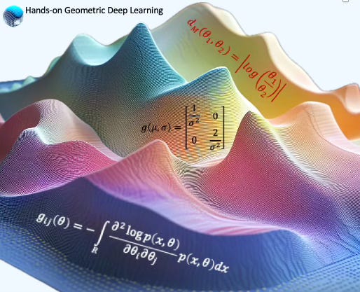
A Fisher-Riemann manifold is a differentiable manifold MM whose points correspond to probability distributions p(x∣θ) from a statistical model parameterized by θ∈Θ⊂Rn, and which is equipped with the Fisher information metric [ref 6].
The Fisher information metric or Fisher-Rao metric is a Riemannian metric defined on the parameter space of a family of probability distributions, constructed using the Fisher information matrix. It remains invariant under reparameterization and is the only Riemannian metric that aligns with the model’s notion of information about its parameters [ref 7].
From the Riemannian metric:
The Fisher information for a continuous probability density function p is defined as
and for discrete distributions,
Under mild regularity conditions, the Fisher Information metric can be re-written
The Fisher information induces a positive semi-definite metric on the parameter manifold, allowing the use of tools from differential/Riemannian geometry.
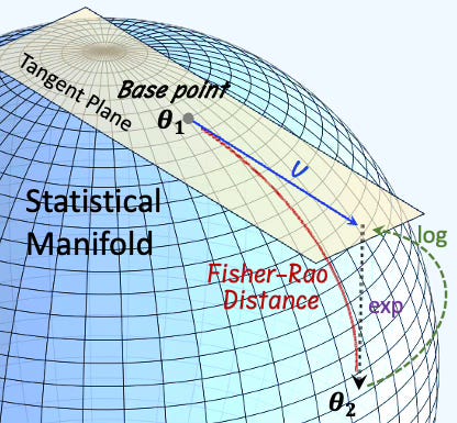
Fig. 1 Visualization of the elements of a statistical manifold
The Fisher metric is invariant under sufficient statistics, making it intrinsic to the statistical model.
⚠️ The terminology found in the literature can be confusing. Strictly speaking the Fisher-Riemann manifold is the manifold of distributions equipped with the Fisher-Rao metric. It is also called the Fisher information manifold or the statistical manifold.
Non-tractable Manifolds
For most statistical manifolds associated with multivariate distributions, geometric properties such as the exponential and logarithm maps, inner product, and distance generally lack closed-form (analytical) expressions.
Both formulas A and B rely on an integral to compute the Fisher-Riemannian metric over a given domain or interval. As a result, for non-tractable statistical manifolds, the lower and upper bounds also known as support of the integral must be specified.
Exponential & Log Maps
In information geometry, an exponential manifold is defined over a statistical model that forms an exponential family. The exponential map at a point θ maps a tangent vector v at θ to a point on the manifold along the geodesic defined by v.
📌 Multi-dimensional statistical manifolds are typically intractable. However, by reducing the number of parameters to one—such as fixing the standard deviation—it becomes possible to derive closed-form expressions for the exponential and logarithm maps.
Exponential Distributions
Probability Density Function
Given a rate parameter θ > 0 the probability density function of the exponential distribution is
Fisher Information Metric
The Riemannian metric associated with the exponential distribution with
Exponential map
Fisher-Rao geodesics correspond to exponential curves in probability space, but the parameterization remains linear in θ, so the exponential map is affine.
logarithm map
In general, the logarithm map is the inverse of the exponential map. Given a base point on the Exponential manifold θ1 that points towards a point θ2:
Geometric Distributions
Probability Density Function
Given the probability of success p at each trial, the probability of success after k trials is
Fisher Information Metric
Exponential Map
Given a tangent vector v and a base point p1 on the Geometric Distribution manifold
Logarithm Map
Given a base point p1 and a point on a Geometric distribution manifold p2
Poisson Distributions
Probability Density Function
Given a Poisson distribution with the expectation λ (rate parameter) events for a specific interval, the probability of k events in the same interval is
Fisher Information Metric
Exponential Map
Given a base point λ1 on the Poisson manifold and a tangent vector v
Logarithm Map
Given a base point λ1 and a point on a manifold λ2
Binomial Distributions with Fixed Draws
Binomial Distribution has a closed form in the case number of draws is fixed.
Probability Density Function
Given a probability distribution of success p in a sequence of n independent experiments.
Fisher Information Metric
The Riemann metric g is defined as
Exponential map
Given a tangent vector v and a base point p1
Logarithm Map
Given a base point p1 and a point on a binomial manifold p2
📌 The computation of the exponential and logarithm map for Normal Distribution is intractable, However, fixing either the mean or standard deviation generates a closed form.
⚙️ Hands-on with Python
Environment
Libraries: Python 3.12.5, PyTorch 2.5.0, Numpy 2.2.0, Geomstats 2.8.0
Source code: geometriclearning/geometry/information_geometry
Evaluation code: geometriclearning/play/cd_statistical_manifold_play.py
The source tree is organized as follows: features in python/, unit tests in tests/,and newsletter evaluation code in play/.
To enhance the readability of the algorithm implementations, we have omitted non-essential code elements like error checking, comments, exceptions, validation of class and method arguments, scoping qualifiers, and import statements.
Our implementation of the evaluation of various statistical manifolds relies on Geomstats Python library [ref 8], introduced in a previous article [ref 9].
📈 Visualization
First let’s briefly review these family of one-dimensional distribution by sampling their parameter and visualizing their probability density functions.
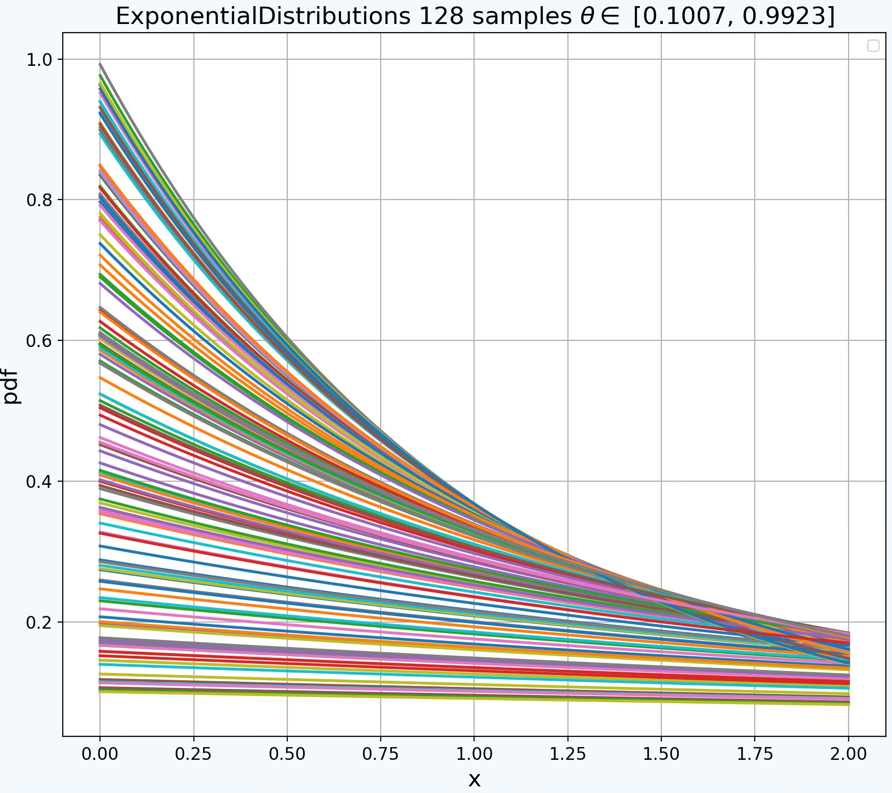
Fig. 2 Family of Exponential Distributions with random samples of the natural parameter θ
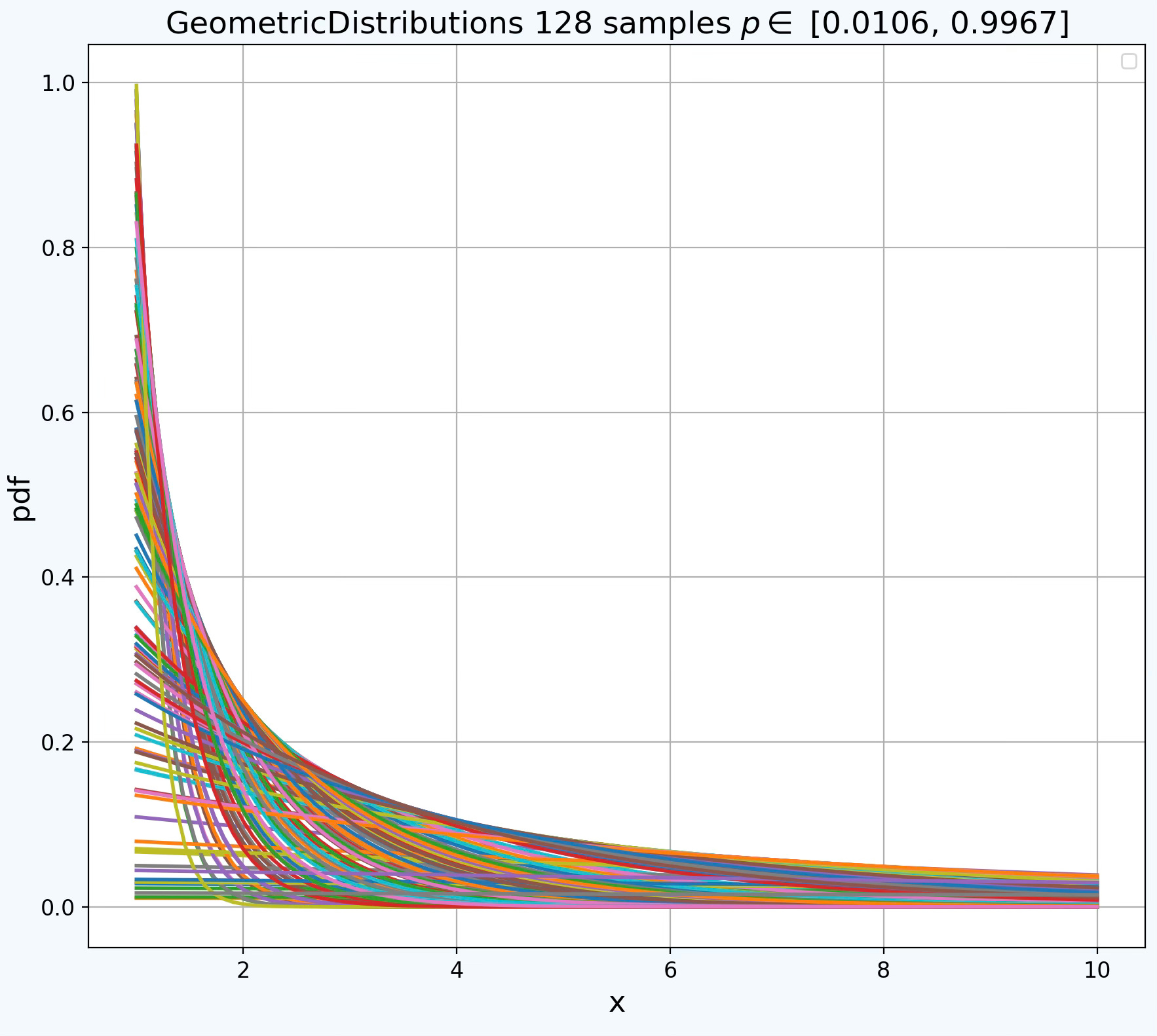
Fig. 3 Family of Geometric Distributions with random samples of the probability of success p
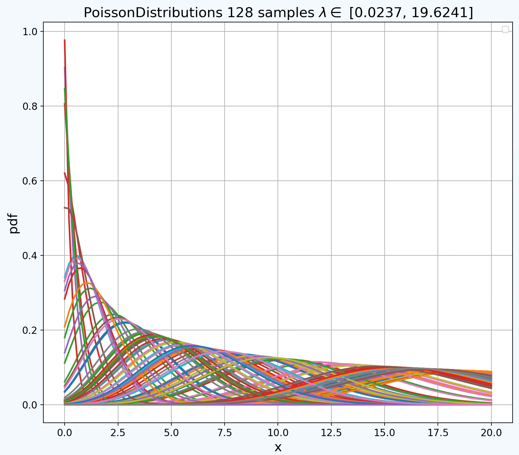
Fig. 4 Family of Poisson Distributions with random samples of the rate parameter λ
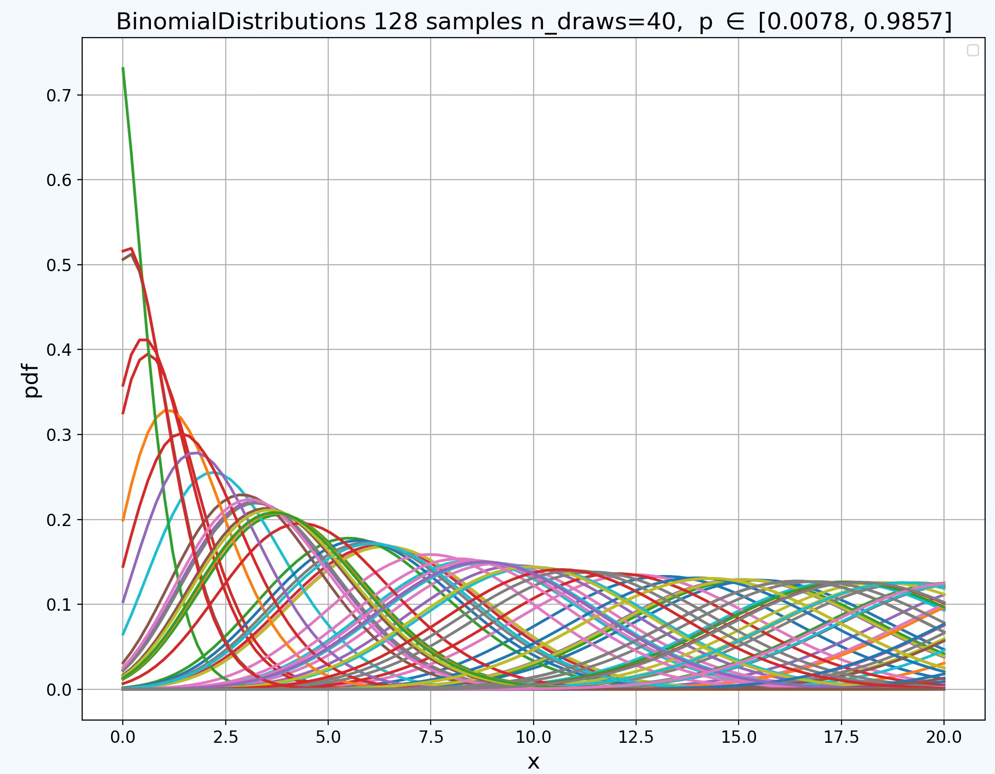
Fig. 5 Family of Binomial Distributions with random samples of probability of success p
🔎 Setup
⏭️ This section guides you through the design and code.
Let’s create a class, CFStatisticalManifold to encapsulates the various operations on the statistical manifolds with closed-form for exponential and logarithm map (Code snippet 1).
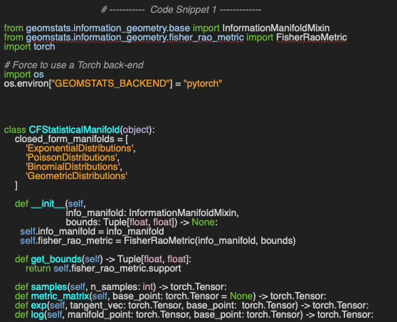
📌 I limit this evaluation to four families of distributions: Exponential, Poisson, Binomial, and Geometric. Several other distributions, like the Bernoulli, also admit closed-form expressions for the exponential and logarithm maps.
The constructor initializes the distribution family on the manifold, info_manifold and sets up a reference to the Fisher-Rao metric provided by Geomstats, fisher_rao_metric, using predefined bounds.
⚠️ Computing the Fisher metric in Geomstats requires either the Autograd or PyTorch backend.
The method belongs (Code snippet 2) checks whether each point lies on the manifold by calling the corresponding belongs method from Geomstats.
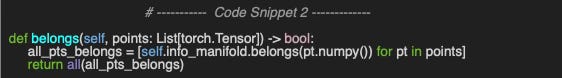
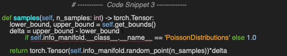
As discussed in a previous article on Riemannian manifolds like the hypersphere, this evaluation depends on the framework’s ability to generate random data points on statistical manifolds, as illustrated in Code snippet 3.
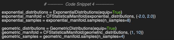
Let’s now put the current implementation of our CFStatisticalManifold class to use, as shown in Code snippet 4.
👉 Evaluation code is available at geometriclearning/play/cd_statistical_manifold_play.py
Output
Exponential Distribution Manifold 8 random samples
tensor([0.8494])
tensor([0.1072])
tensor([0.6849])
tensor([0.3375])
tensor([0.1472])
tensor([0.4026])
tensor([0.4321])
tensor([0.2589])
Geometric Distribution Manifold 4 random samples
tensor([0.4640])
tensor([0.6331])
tensor([0.5167])
tensor([0.7566])
🔎 Fisher Information Metric
The computation of the exponential and logarithm maps, distance, and inner product relies on the Fisher-Rao metric g. The metric_matrix method (Code Snippet 5) implements the computation of this metric at a specified point on the manifold, referred to as the base_point. If no base point is provided, the method selects one at random.
In all cases, the base point is first validated to ensure it lies on the manifold. The actual metric computation is then performed using a call to the Geomstats API.
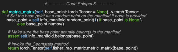
Let’s compute the Fisher metric for the Exponential and Poisson distributions. Since these are univariate distributions, both the points on the manifold and the resulting metric are represented as 1×1 matrices
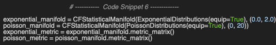
Output:
Exponential Distribution Fisher metric: tensor([[1.0288]])
Poisson Distribution Fisher metric: tensor([[3.1438]])
🔎 Exponential Maps
Let’s implement the computation of endpoint locations on the manifold, (method exp) given a base point and a tangent vector, for these four closed-form manifolds using the formulas defined in the previous section for the exponential map (Code snippet 7).
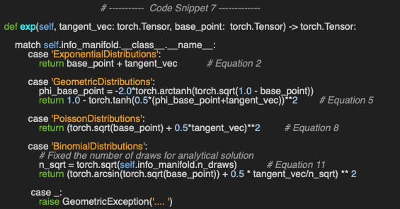
Finally, we leverage the method exp to compute the end points on the Exponential and Geometric manifolds, exponential_end_point (resp. geometric_end_point).
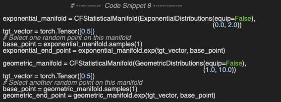
Output
Exponential Distribution Manifold End point: tensor([0.8868])
Geometric Distribution Manifold End point: tensor([0.9326])
🔎 Logarithm Maps
We implement the formulas to compute the tangent vector given a base point and another point on the manifold for the same closed-form statistical manifolds (method log in code snippet 9).
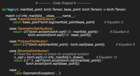
Exponential Distribution Manifold Tangent Vector
Base:tensor([0.4471]) to:tensor([0.7085]): tensor([0.2059])
Geometric Distribution Manifold Tangent Vector
Base:tensor([0.9392]) to:tensor([0.7573]): tensor([-5.7546])
🧠 Key Takeaways
✅ Information geometry is a field of mathematics that applies differential geometry to study the structure of statistical models. It extends Riemannian geometry to the space of probability density functions, enabling a geometric approach to statistical inference.
✅ While multivariate statistical manifolds often lead to intractable exponential and logarithm maps, univariate distributions typically admit closed-form expressions.
✅ In some cases, fixing one or more parameters of a distribution can simplify an otherwise intractable manifold into a closed-form representation.
✅ The Geomstats library in Python provides a practical toolkit for exploring, analyzing, and applying core concepts of information geometry, though closed-form manifolds can often be computed manually with relative ease.
📘 References
Differential Geometric Structures W. Poor - Dover Publications, New York 1981
Introduction to Smooth Manifolds J. Lee - Springer Science+Business media New York 2013
What is Fisher Information? YouTube - Ian Collings
An Elementary Introduction to Information Geometry F. Nielsen - Sony Computer Science Laboratories.
🛠️ Exercises
What is the geometric structure of a point on a statistical manifold defined by n parameters?
What is the Fisher information metric of the normal distribution when the standard deviation is fixed and not treated as a parameter?
Can you implement the Fisher information metric for a normal distribution with a constant, fixed standard deviation?
Can you compute the Fisher-Rao metric manually for the exponential distribution manifold?
👉 Answers
💬 News & Reviews
This section focuses on news and reviews of papers pertaining to geometric deep learning and its related disciplines.
Paper Reviews: Manifold Matching via Deep Metric Learning for Generative Modeling M. Dai, H. Hang
This study advances the recent progress in blending geometry with statistics to enhance generative models. It proposes a novel method for identifying manifolds within Euclidean spaces for generative models like variational encoders and GANs through two neural networks:
Data generator sampling data on the manifold
Metric generator learning geodesic distances.
Metric learning:
The metric generator produces a pullback of the Euclidean space while the data generator produces a push forward of the prior distribution. The algorithm is described with easy-to-follow pseudo code.
The method is tested on unconditional ResNet image creation and GAN-based image super-resolution, showing improved Frechet Inception Distance and perception scores.
This paper will be especially of interest to engineers already familiar with GANs and Frechet metric.
Expertise Level
⭐ Beginner: Getting started - no knowledge of the topic
⭐⭐ Novice: Foundational concepts - basic familiarity with the topic
⭐⭐⭐ Intermediate: Hands-on understanding - Prior exposure, ready to dive into core methods
⭐⭐⭐⭐ Advanced: Applied expertise - Research oriented, theoretical and deep application
⭐⭐⭐⭐⭐ Expert: Research , thought-leader level - formal proofs and cutting-edge methods.
Patrick Nicolas is a software and data engineering veteran with 30 years of experience in architecture, machine learning, and a focus on geometric learning. He writes and consults on Geometric Deep Learning, drawing on prior roles in both hands-on development and technical leadership. He is the author of Scala for Machine Learning (Packt, ISBN 978-1-78712-238-3) and the newsletter Geometric Learning in Python on LinkedIn.
Appendix
Computation of the Fisher matrix for Normal distribution.
Very well explained and indeed a gem post.