

Topological Lifting of Graph Neural Networks
Expertise Level ⭐⭐⭐⭐

At some point you’ve probably hit the limits of standard Graph Neural Networks. What if you could lift your graph to a richer topological domain to explore, and ultimately improve node classification or link prediction?
(🔎) Optional source code section
🎯 Why this matters
Purpose: In the previous article [ref 4], we used TopoNetX to build simplicial complexes and compute the Hodge Laplacian. The question now is: how do we lift an existing graph dataset into a simplicial complex?
Audience: For data scientists and engineers curious about Topological Deep Learning and ways to push past Graph Neural Networks limits.
Value: Construct a simplicial complex from an existing graph dataset with the Hodge Laplacian, illustrated in PyTorch Geometric and TopoNetX libraries
🎨 Modeling & Design Principles
Overview
There are few fully specified simplicial-complex datasets for exploring these topological methods and assessing their impact on prediction and classification. One practical approach is to derive faces (triangles) from an existing graph and then compute feature vectors for nodes, edges, and faces from the graph’s geometry.
⚠️ The literature uses varied terms for per-node features—‘node representations,’ ‘node embeddings,’ etc.—and similarly for edges and faces. In this article, we use the term feature vector uniformly for any simplicial element.
One key benefit of this approach is that can be fully automated and leverage existing Python libraries; NetworkX, PyTorch Geometric (PyG) and TopoX. These libraries have been described in previous articles [ref 1, 2, 3].
Constructing Simplicial Complexes
Let’s review common ways to build Graph and Simplicial Neural Networks (see Fig. 1).
Graph Neural Networks.
As covered in earlier articles [ref], GNNs are typically built from PyTorch Geometric datasets that include node features and, optionally, edge features [A}. You can also start with a bare graph (e.g., a NetworkX graph) and attach node features to train a GNN [B].
Simplicial Neural Networks.
SNNs can be instantiated directly from a fully specified simplicial complex [C]. Alternatively, you can augment graph data by adding faces (e.g., triangles) and either assigning feature vectors to edges and faces [D] or using edges and faces in the message passing/aggregation.
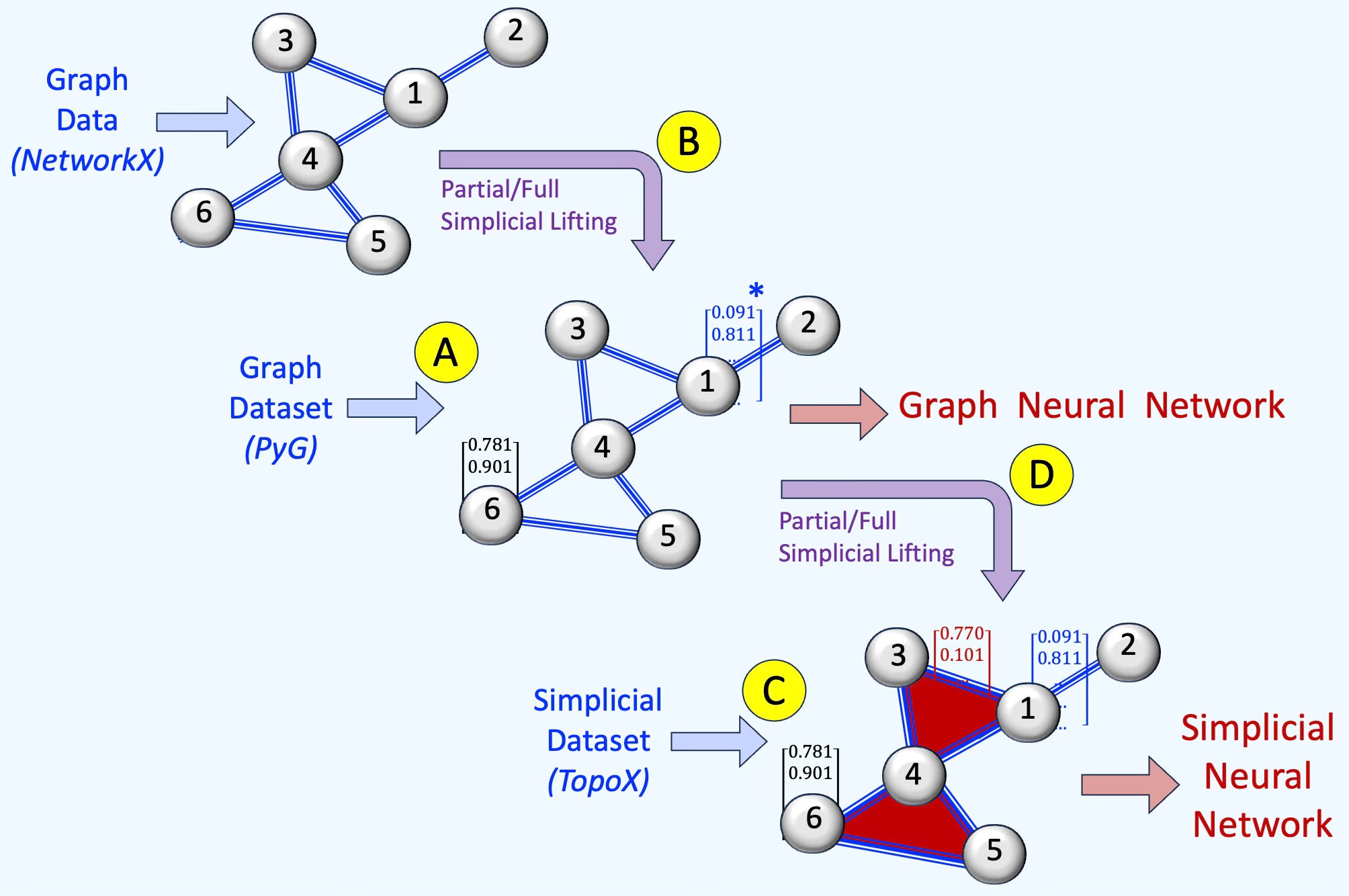
Fig. 1 Illustration of various scenarios to build or lift a graph into a simplicial complex.
The simplicial complex has been introduced in a previous article [ref 4]
The table below summarizes how to infer node, edge, and face features when they aren’t provided by the PyTorch Geometric or TopoX datasets.
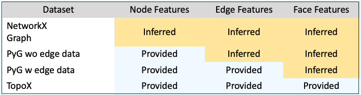
Table 1. Summary of completion of a given simplicial complex data representation.
The conversion of a graph data into a simplicial complex is known as topological lifting or simply lifting.
Simplicial Lifting
Node, edge and face representation (or embedding) generated through Hodge Laplacian and incidence matrices are very sparse.
📌 Full Simplicial lifting assigns signal/features to faces or triangles. Partial Simplicial lifting uses topological domains in the message passing and aggregation only (e.g., L1 Hodge Laplacian). This article applies Partial Simplicial Lifting.
We split the automated pipeline for building a fully functional simplicial complex from a graph into five steps:
Select/load a fully specified graph (structure only; no embeddings)
Add faces (e.g., triangles/tetrahedra)
Generate data from incidence matrices
Generate edge data for message passing/aggregation via the Hodge 1-Laplacian
Generate face data for message passing/aggregation via the Hodge 2-Laplacian.
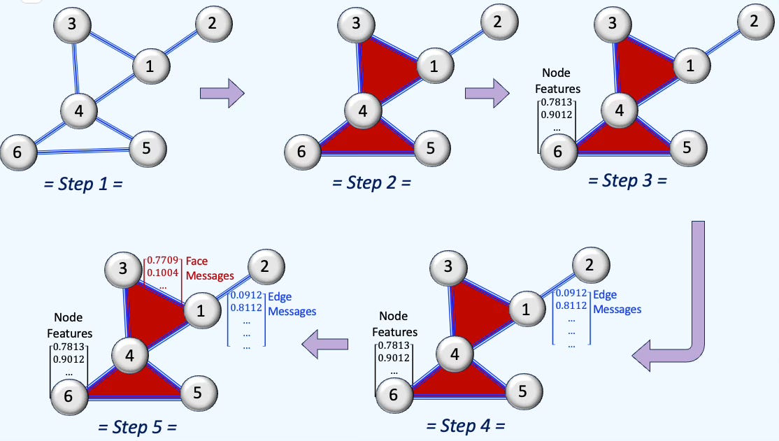
Fig. 2 Steps to generate a simplicial complex from a graph using partial simplicial lifting
Let’s dig into the mathematical inner workings for extracting edge and face feature vector to generate simplicial complexes. The procedures relies on the extraction of incidence matrices and Hodge Laplacian [ref 5].
The k smallest eigenvectors of L1 (Hodge Laplacian for edges) and L2 (Hodge Laplacian for faces/triangles) give you two structure-aware positional encodings that can be concatenated.
The process can be broken down in 4 stages:
Stage 1: Build incidence matrices B1 (node x edge incidence) and B2 (edge x face incidence) while preserving orientation (+1 for edge u →v, -1 for edge v → u)
Stage 2: Compute the edge Hodge Laplacian L1 and face Hodge Laplacian L2 as
Stage 3: Extract the first k smallest eigenvalues and compute their associated eigenvectors.
Stage 4: Convert eigenvectors into features (L1 => edge feature set, L2 => face feature set)
Stage 5: Concatenate these features to features extracted from input graph data.
There are variant of this method that consists of
Stage 2: Normalizing the Hodge Laplacians
Stage 5: Replace concatenation of features by transformation such as trigonometric lift
📌 Hodge Laplacian and Manifolds: The spectrum of the Hodge Laplacian encodes topological structure on manifolds and simplicial complexes and is tied to sectional curvature; suitable curvature assumptions can yield small eigenvalues.
⚙️ Hands‑on with Python
Environment
Libraries: Python 3.12.5, PyTorch 2.5.0, Numpy 2.2.0, Networkx 3.4.2, TopoNetX 0.2.0
Source code: Features: geometricLearning/topology/simplicial/graph_to_simplicial_complex.py
Evaluation code: geometriclearning/play/graph_to_simplicial_complex_play.py
The source tree is organized as follows: features in python/, unit tests in tests/, and newsletter specific evaluation code in play/.
To enhance the readability of the algorithm implementations, we have omitted non-essential code elements like error checking, comments, exceptions, validation of class and method arguments, scoping qualifiers, and import statements.
🔎 Setup
⏭️ This section guides you through the design and code
Let’s wrap the process of lifting (or converting) a graph into a Simplicial in a class, GraphToSimplicialComplex.
📌 The constructor doesn’t require a NetworkX graph, nx_graph. You can pass either a fully defined dataset instance or a dataset identifier.
The arguments of the constructors (code snippet 1) are
nx_graph: NetworkX graph is provided or None if the graph has to be created from the dataset
dataset: A PyTorch Geometric dataset if defined (T: torch_geometric.util.data.Dataset) or name of the dataset (T: str)
lifting_method: One of the lifting methods provided by TopoNetX library; graph_to_clique_complex, graph_to_neighbor_complex or weighted_graph_to_vietoris_rips_complex.
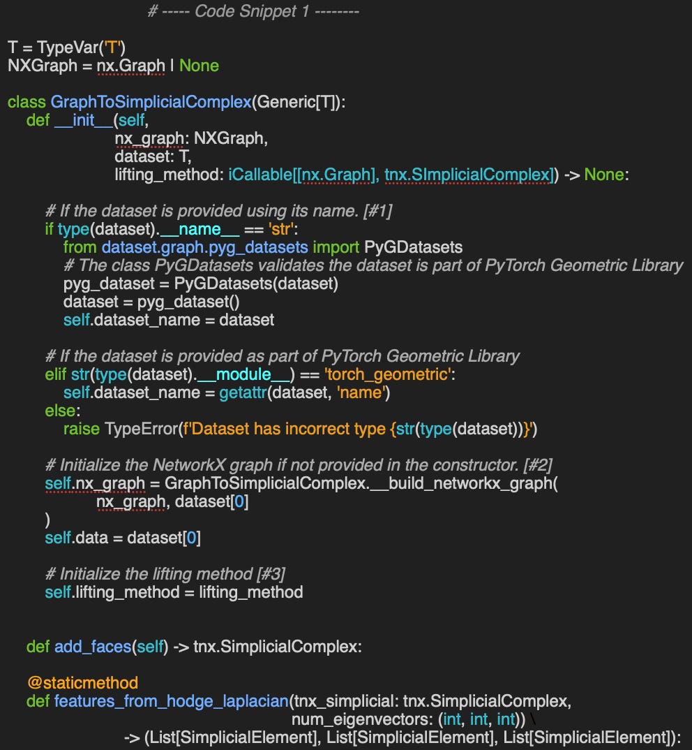
The constructor first inspects the argument dataset: if it is supplied as a type, the dataset is instantiated; if not, its name or identifier is extracted [#1]. Next, if no NetworkX graph (nx.Graph) is given, one is created from the dataset [#2]. A short description of this procedure is provided in the appendix. Finally, the constructor determines selects the lifting method ]#3].
The list of PyTorch Dataset has been described in a previous article [ref 6].
📌 We use generic type (TypeVar(‘T’)) for backward compatibility with Python version earlier than 3.12
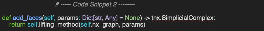
🔎 Adding Faces
⏭️ This section guides you through the design and code
The next step is to automatically augment the existing graph with its faces. The method add_faces invokes any of the TopoNetX method that lift an existing graph to a clique, neighbors or Vietoris-Rips complex.
The TopoNetX library offers three approaches for this task [ref 7]:
graph_to_clique_complex: Enumerates all cliques in a NetworkX graph and updates its nodes and edges accordingly.
graph_to_neighbor_complex: Constructs the complex by loading the neighborhood of each node.
weighted_graph_to_vietoris_rips_complex: Builds a Vietoris-Rips complex on an existing weighted graph.
📌 The Vietoris-Rips complex is beyond the scope of this article and therefore won’t be evaluated.
We write two wrapper methods lift_from_graph_cliques and lift_from_graph_neighbors with the signature as required by the constructor
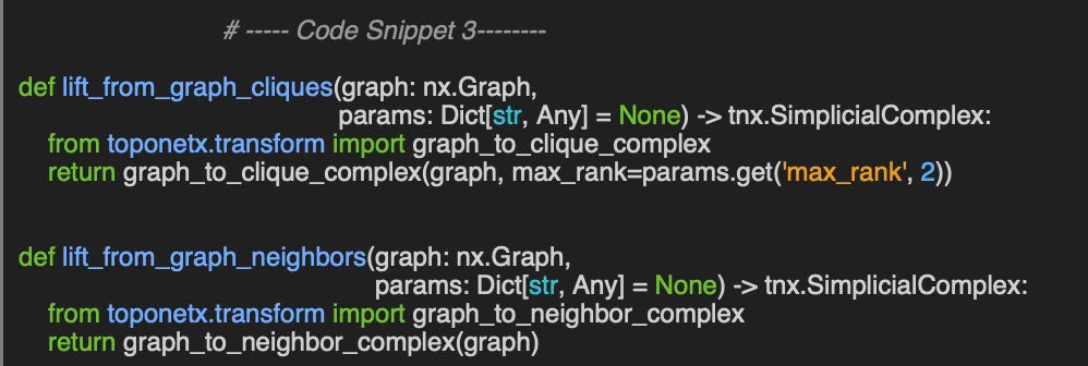
The parameter max_rank defines the level of simplex (0 for node, 1 for edge, 2 for triangles/faces, 3 for Tetrahedrons).
👉 Test code: geometriclearning/tutorial/_graph_to_simplicial_complex.py
Let’s add faces (max_rank=2) to Cora and KarateClub PyTorch Geometric graph data as illustrated in the code snippet 4. We select a different lifting methods for each of the data set invoked through its name.
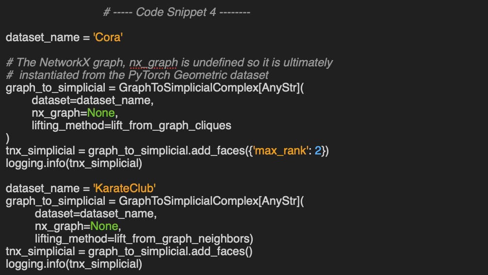
Output:
Simplicial Complex with shape (2708, 5278, 1630) and dimension 2

Simplicial Complex with shape (34, 343, 1787, 6106, 15852, 32322, 52610, 69061, 73489, 63438, 44267, 24764, 10949, 3740, 952, 170, 19, 1) and dimension 17
⚠️ Lifting via node neighborhoods captures more information at the expense of a substantially larger number of nodes and edges, increasing computational cost.
🔎 Adding Features
⏭️ This section guides you through the design and code
The last stages consist of generating the features using the Hodge Laplacian described in previous article [ref 5] and implemented in the method features_from_hodge_laplacian.
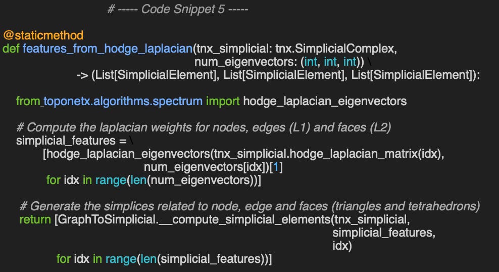
The method takes two arguments:
tnx_simpicial: graph augmented with faces, as a simplicial complex
num_eigenvectors: k, l and m smallest values used in Hodge Laplacian to generate k node, l edge and m face features
The eigenvectors are computed through the TopoNetX method hodge_laplacian_eigenvectors [ref 8].
We now have what we need to generate the simplicial elements (nodes, edges, faces) via the GraphToSimplicialComplex class in three straightforward steps. The code snippet 6 implements the 5 stages described in the Modeling & Design Principle section.
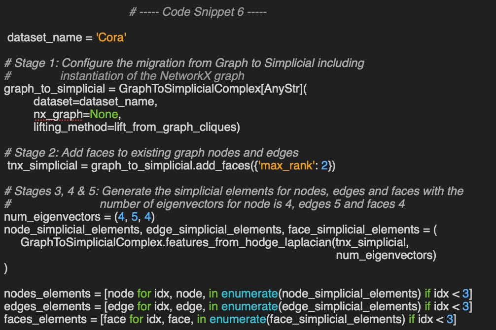
Here are the outputs for the first three nodes—and their associated edges and faces—from the Cora dataset.
Nodes: 3, Edges: 3, Faces: 3 eigenvectors
Simplicial nodes:
[-0.00183, -0.00577, -0.0072], (0,)
[-0.00183, -0.00577, -0.0072], (1,)
[-0.00183, -0.00577, -0.0072], (2,)
Simplicial edges:
[-0.01275, 0.02554, -0.00548], (0, 633)
[0.01452, -0.02043, -0.00536], (0, 1862)
[-0.00177, -0.00511, 0.01085], (0, 2582)
Simplicial faces:
[0.0, 0.0, -0.0], (0, 1862, 2582)
[0.00413, -0.0203, 0.0], (4, 1016, 1256)
[-0.00413, 0.0203, -0.0], (4, 1016, 2176)

Nodes: 5, Edges: 6, Faces: 5 eigenvectors
Simplicial nodes:
[0.00386, -0.00093, -0.00093, -0.00422, -0.003], (0,)
[0.00386, -0.00093, -0.00093, -0.00422, -0.003], (1,)
[0.00386, -0.00093, -0.00093, -0.00422, -0.003], (2,)
Simplicial edges:
[-0.03155, 0.0189, -0.01599, -0.00045, -5e-05, 1e-04], (0, 633)
[0.02973, -0.01424, 0.01506, -8e-05, 3e-05, -1e-05], (0, 1862)
[0.00182, -0.00467, 0.00093, 0.00063, 0.0004, -0.00035], (0, 2582)
Simplicial faces:
[0.0, 0.0, -0.0, 0.0, -0.0], (0, 1862, 2582)
[0.01416, 0.01416, -0.02223, 0.01926, -0.00849], (4, 1016, 1256)
[-0.01416, -0.01416, 0.02223, -0.01926, 0.00849], (4, 1016, 2176)

Nodes: 10, Edges: 9, Faces: 9 eigenvectors
Simplicial nodes:
[6e-05, 0.00296, -0.00229, 0.00016, 0.00016, -0.00449, 0.00359, -0.00047, 0.00174, 0.00095], (0,)
[6e-05, 0.00296, -0.00229, 0.00016, 0.00016, -0.00449, 0.00359, -0.00063, 0.00079, -0.00025], (1,)
[6e-05, 0.00296, -0.00229, 0.00016, 0.00016, -0.00449, 0.00359, -0.0005, 0.00057, 0.00041], (2,)
Simplicial edges:
[0.01814, -0.01984, 0.00022, 0.00022, 0.00133, 0.00468, 0.00468, -0.00303, -0.00303], (0, 633)
[-0.01446, 0.01925, 0.00139, 0.00139, -0.00357, -0.00076, -0.00076, 0.00251, 0.00251], (0, 1862)
[-0.00368, 0.00059, -0.00161, -0.00161, 0.00224, -0.00391, -0.00391, 0.00053, 0.00053], (0, 2582)
Simplicial faces:
[0.0, 0.0, 0.0, -0.0, 0.0, 0.0, 0.0, 0.0, 0.0], (0, 1862, 2582)
[0.02101, -0.00813, 0.00754, -0.00689, -0.00293, -0.00293, -0.00337, 0.00264, 0.00264], (4, 1016, 1256)
[-0.02101, 0.00813, -0.00754, 0.00689, 0.00293, 0.00293, 0.00337, -0.00264, -0.00264], (4, 1016, 2176
Latency Consideration
The size of the graph features and nodes has a significant impact on the duration of the generation of edges and faces as described in table 2.
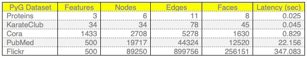
Table 2. Latency for generation of simplicial elements from some graph datasets bundled with PyTorch Geometric library
🧠 Key Takeaways
✅ Lifting an input graph to a simplicial complex consists of (i) identifying faces and (ii) assigning weights to the resulting simplices.
✅ These weights may be computed from edge and face incidence operators and their Hodge–Laplacians.
✅ The TopoNetX library supports three lifting strategies—clique complexes, neighborhood-based complexes, and weighted Vietoris–Rips complexes.
✅ Lifting via node neighborhoods captures more information at the expense of significant computational cost.
✅ The complexity of the construction grows very significantly with the size of the complex.
📘 References
NetworkX Hands-on Geometric Deep Learning - 2025
TopoX Hands-on Geometric Deep Learning - 2025
Exploring Simplicial Complexes for Deep Learning Hands-on Geometric Deep Learning - 2025
Hodge-Laplacian Hands-on Geometric Deep Learning - 2025
🛠️ Exercises
Q1: Which class in the TopoNetX library represents simplicial complexes?
Q2: What are Hodge–Laplacians?
Q3: Could you show an example of constructing a NetworkX graph from a PyTorch Geometric dataset?
Q4: Compared to a clique-based lifting, does a neighborhood-based lifting typically produce a higher-dimensional simplicial complex (i.e., more or higher-order simplices)?
💬 News & Reviews
This section focuses on news and reviews of papers pertaining to geometric deep learning and its related disciplines.
Paper Review: TopoTune: A Framework for Generalized Combinatorial Complex Neural Networks M. Papillon, G. Bernardez, C. Battiloro, N. Miolane 2025
Graph Neural Networks (GNNs) can be seen as a 1-dimensional special case within the broader framework of Topological Deep Learning, which generalizes deep learning to more expressive relational structures beyond graphs. This paper introduces a library that extends PyTorch to support combinatorial complexes, much like how PyTorch Geometric supports GNNs.
After introducing the concept of combinatorial complexes, the authors adapt the message-passing paradigm to operate on these generalized topological structures, which are ultimately represented as Hasse graphs. The proposed Generalized Combinatorial Complex Neural Network (GCCNN) is designed to be equivariant under label permutations and both node-level (intra-neighborhood) and cell-level (inter-neighborhood) permutations.
The accompanying library, TopoTune, builds on top of existing topological libraries such as TopoNetX and TopoModelX, and provides tools to convert PyTorch Geometric graph datasets into topological datasets suitable for higher-order learning.
The performance of GCCNN is evaluated against variants of Combinatorial Complex Neural Networks (CCNNs) based on well-known GNN architectures like GraphSAGE, Graph Convolutional Networks, and Graph Attention Networks. Experiments are conducted on datasets such as MUTAG, NCI0x, PROTEINS, as well as common PyTorch Geometric benchmarks like Cora and CiteSeer. The results show that GCCNN consistently outperforms CCNN models, especially on standard GNN datasets.
Notes:
Source code for TopoTune is available on GitHub
Basic knowledge in Graph Neural Network and Topological Data Analysis recommended.
Expertise Level
⭐ Beginner: Getting started - no knowledge of the topic
⭐⭐ Novice: Foundational concepts - basic familiarity with the topic
⭐⭐⭐ Intermediate: Hands-on understanding - Prior exposure, ready to dive into core methods
⭐⭐⭐⭐ Advanced: Applied expertise - Research oriented, theoretical and deep application
⭐⭐⭐⭐⭐ Expert: Research , thought-leader level - formal proofs and cutting-edge methods.
Patrick Nicolas is a software and data engineering veteran with 30 years of experience in architecture, machine learning, and a focus on geometric learning. He writes and consults on Geometric Deep Learning, drawing on prior roles in both hands-on development and technical leadership. He is the author of Scala for Machine Learning (Packt, ISBN 978-1-78712-238-3) and the newsletter Geometric Learning in Python on LinkedIn.