

Uniform Manifold Approximation & Projection
Expert level: ⭐⭐⭐

Are you frustrated with the linear assumptions of Principal Component Analysis (PCA) or losing the global structure and relationships in your data with t-SNE?
Leveraging Riemannian geometry, Uniform Manifold Approximation and Projection (UMAP) might be the solution you're looking for.
🎯 Why this Matters
Purpose: Address the limitations of Principal Component Analysis (PCA) and t-SNE projection.
Audience: Data scientists and engineers with basic understanding of dimension reduction.
Value: Learn to apply Uniform Manifold Approximation and Projection method as a reliable non-linear dimensionality reduction technique that preserve the global distribution over low dimension space.
🎨 Modeling & Design Principles
Overview
Dimension reduction algorithms can be classified into two categories:
Models that maintain the global pairwise distance structure among all data samples, such as Principal Component Analysis (PCA) and Multidimensional Scaling (MDS).
Models that preserve local distances, including t-distributed Stochastic Neighbor Embedding (t-SNE) and Laplacian Eigenmaps.
Uniform Manifold Approximation and Projection (UMAP) leverages research done for Laplacian eigenmaps to tackle the problem of uniform data distributions on manifolds by combining Riemannian geometry with advances in fuzzy simplicial sets [ref 1].
t-SNE is considered the leading method for dimension reduction in visualization. However, compared to t-SNE, UMAP maintains more of the global structure and offers faster run time performance.
Both t-SNE and UMAP are Non-linear Dimension Reduction techniques
t-SNE
t-SNE is a widely used technique for reducing the dimensionality of data and enhancing its visualization. It's often compared to PCA (Principal Component Analysis), another popular method. This article examines the performance of UMAP and t-SNE using two well-known datasets, Iris and MNIST.
t-SNE is an unsupervised, non-linear technique designed for exploring and visualizing high-dimensional data [ref 2]. It provides insights into how data is structured in higher dimensions by projecting it into two or three dimensions. This capability helps reveal underlying patterns and relationships, making it a valuable tool for understanding complex datasets.
UMAP
UMAP, developed by McInnes and colleagues, is a non-linear dimensionality reduction technique that offers several benefits over t-SNE, including faster computation and better preservation of the global structure of the data.
Benefits
Ease of Use: Designed to be easy to use, with a simple API for fitting and transforming data.
Scalability: Can handle large datasets efficiently.
Flexibility: Works with a variety of data types and supports both supervised and unsupervised learning.
Integration: Integrates with other Python scientific computing libraries in Python, such as Numpy, PyTorch and Scikit-learn.
The algorithm behind UMAP involves:
Constructing a high-dimensional graph representation of the data.
Capturing global relationships within the data.
Encoding these relationships using a simplicial set.
Applying stochastic gradient descent (SGD) to optimize the data's representation in a lower dimension, akin to the process used in autoencoders.
This method allows UMAP to maintain both local and global data structures, making it effective for various data analysis and visualization tasks.
For the mathematically inclined, the simplicial set captures the local and global relationships between two points xi and xj as:
with sigma parameters as the scaling factor for each data point.
The cost function for all the points xi with their representation yi is
Python module is installed through the usual pip utility.
pip install umap-learn
The reader is invited to consult the documentation [ref 3].
⚙️ Hands-on with Python
Environment
Libraries: Python 3.11, SciKit-learn 1.5.1, Matplotlib 3.9.1, umap-learn 0.5.6
Source code: geometriclearning/play/umap_play.py
Note: To enhance the readability of the algorithm implementations, we have omitted non-essential code elements like error checking, comments, exceptions, validation of class and method arguments, scoping qualifiers, and import statements.
Geomstats is an open-source, object-oriented library following Scikit-Learn’s API conventions to gain hands-on experience with Geometric Learning. It is described in article Introduction to Geomstats for Geometric Learning
Data
Let's consider the two datasets used for this evaluation (code snippet 1):
MNIST: The MNIST database consists of 60,000 training examples and 10,000 test examples of handwritten digits. This dataset was originally created by Yann LeCun [ref 4].
IRIS: This dataset includes 150 instances, divided into three classes of 50 instances each, with each class representing a different species of iris plant [ref 5].
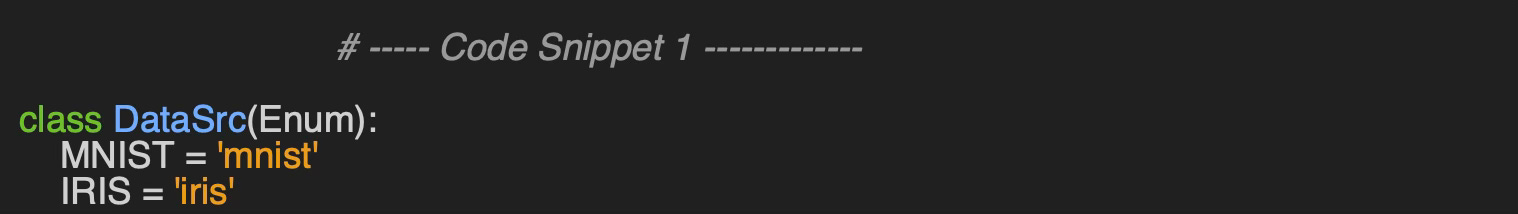
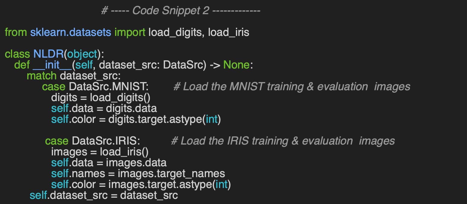
First, I implement a data set loader - class NLDR for Non-linear Dimension Reduction - for these two data sets using sklearn datasets module.
🔎 Evaluation
t-SNE Evaluation Code
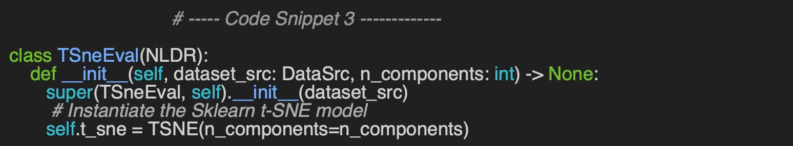
Let's wrap the evaluation of t-SNE algorithm for IRIS and MNIST data in a class TSneEval. The constructor initializes the Scikit-learn class TSNE with the appropriate number of components (dimension 2 or 3). The class TSneEval inherits for sklearn data loaders by subclassing NLDR.
The evaluation method, __call__, utilizes the Matplotlib library to visualize data clusters. It generates plots to display the clusters for each digit in the MNIST dataset and for each flower category in the Iris dataset.
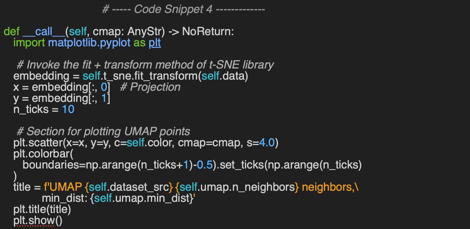
The simple previous code snippet 4 produces the t-SNE plots for MNIST and IRIS data sets.
Output for MNIST Dataset
First let's look at the 10 data clusters (1 per digit) in a two and 3 dimension plot.
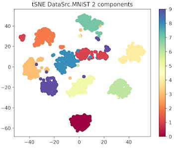
Fig. 1 2-dimension t-SNE for MNIST data set
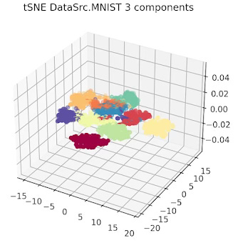
Fig. 2 3-dimension t-SNE for MNIST data set
Output for IRIS Dataset
The data related to each of the 3 types or Iris flowers are represented in 2 and 3 dimension plots.
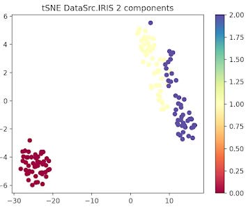
Fig. 3 2-dimension t-SNE for IRIS data set
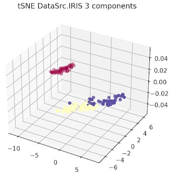
Fig. 4 3-dimension t-SNE for IRIS data set
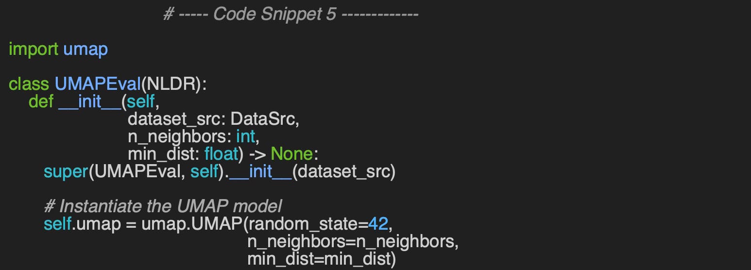
UMAP Evaluation Code
We follow the same procedure for UMAP visualization as we do for t-SNE. The constructor of the UMAPEval wrapper class initializes the UMAP model with the specified number of neighbors (n_neighbors) and minimum distance (min_dist) parameters, which are used to represent the data.
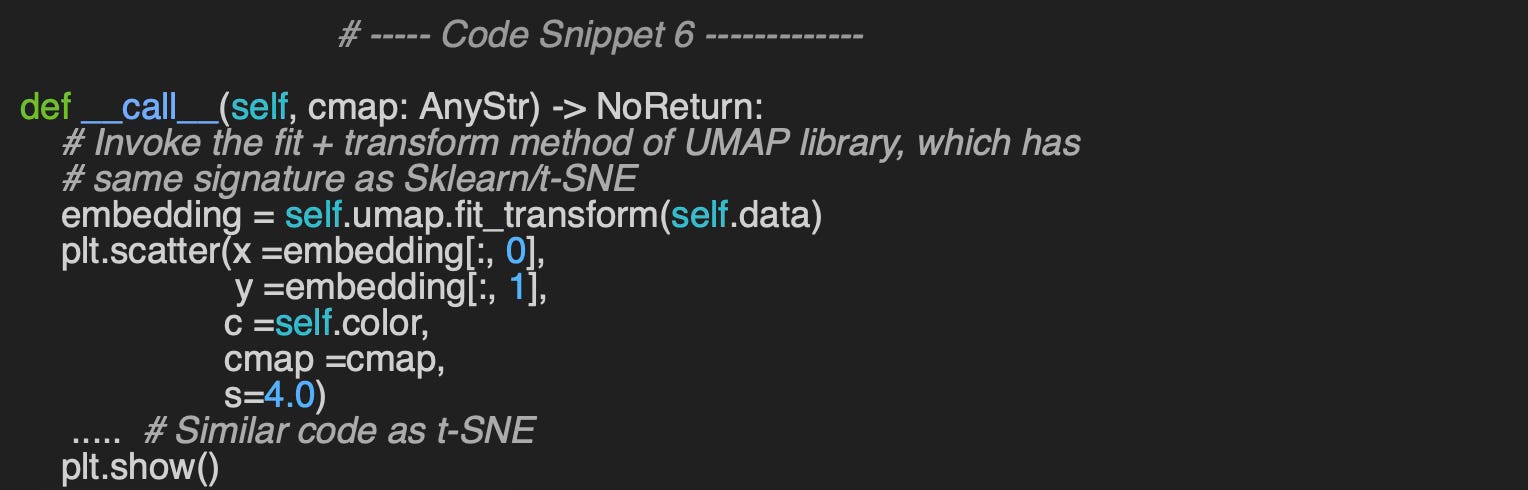
Similar to the t-SNE evaluation, the __call__ method uses the Matplotlib library to visualize data clusters (code snippet 6).
Output for MNIST Dataset
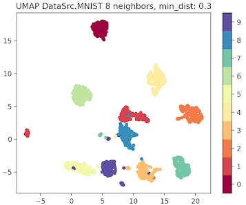
Fig. 5 UMAP plot for MNIST data with 8 neighbors and min distance 0.3
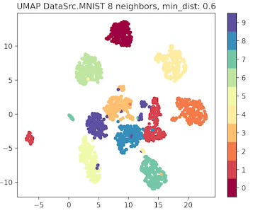
Fig. 6 UMAP plot for MNIST data with 8 neighbors and min distance 0.6
Output for IRIS dataset
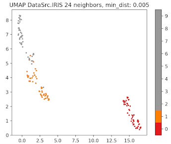
Fig. 8 UMAP plot for IRIS data with 24 neighbors and min distance 0.005
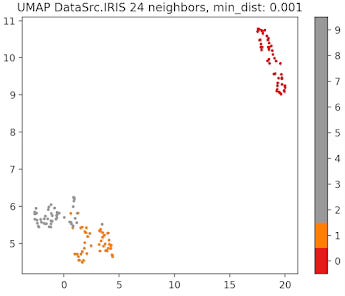
Fig. 9 UMAP plot for IRIS data with 24 neighbors and min distance 0.001
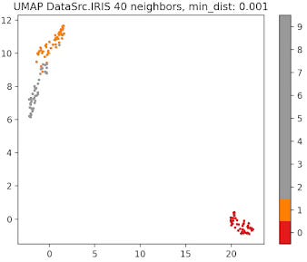
Fig. 10 UMAP plot for IRIS data with 40 neighbors and min distance 0.001
Parameters Tuning 💎
Number of Neighbors (n_neighbors)
The parameter that defines the number of neighbors in UMAP, n_neighbors, determines the balance between global and local distances in the data visualization. A smaller number of neighbors means the local neighborhood is defined by fewer data points, which is ideal for detecting small clusters and capturing fine details. On the other hand, a larger number of neighbors helps in capturing broader, global patterns, but it may oversimplify the local relationships, potentially missing finer details in the data.
Compactness in Low Dimension (min_dist)
This parameter plays a crucial role in determining the appearance of the low-dimensional representation, specifically affecting the clustering and spacing of data points.
A small min_dist value allows UMAP to pack points closer together in the low-dimensional space. It emphasizes the preservation of local structure and can make clusters more distinct. A larger min_dist value enforces a minimum separation between points in the low-dimensional space. UMAP visualizations with a large min_dist may show less clustering and more continuous distributions of data points.
The choice of min_dist thus influences the trade-off between preserving local versus global structures.
🧠 Key Takeaways 💎
✅ The umap-learn library is a great tool to generate embeddings and clusters using Uniform Manifold Approximation & Projection model.
✅ t-SNE is highly effective for revealing clusters in high-dimensional spaces and visualizing 2D and 3D embeddings. However, it comes with significant computational costs and requires considerable time to fine-tune its parameters.
✅ UMAP generates highly meaningful low-dimensional embeddings that align well with clusters. It outperforms t-SNE in preserving both local and global similarities, though tuning its parameters can be challenging.
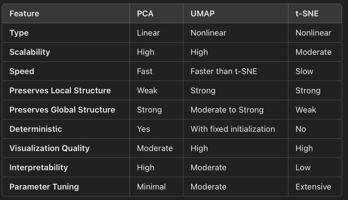
✅ A summary of features of PCA, t-SNE and UMAP models
📘 References
🛠️ Exercises 💎
The aim of these fun, short questions is to highlight key concepts from this article that you may have overlooked.
Q1: What are the two primary categories of models used for feature reduction while preserving distances?
Q2: What formula does UMAP use to calculate the similarity between two points, x & y?
Q3: What is the role of the n_components parameter in t-SNE?
Q4: What are the two key configuration parameters in UMAP?
Q5: How does decreasing min_dist affect the UMAP visualization?
👉 Answers
💬 News & Reviews 💎
This section is focused on news and reviews of papers pertaining to geometric deep learning and its related disciplines.
Review paper: Exploring the Manifold of Neural Networks Using Diffusion Geometry E. Abel & all, 2024
The goal of this ambitious research is to utilize the Potential of Heat-diffusion for Affinity-based Transition Embedding(PHATE) to design a manifold of neural networks, where hyperparameters and architectures are sampled from the manifold.
The key concepts are:
PHATE: A diffusion-based method that preserves an information distance and captures manifolds in very low dimensions, offering an alternative to t-SNE.
Manifold (or landscape) of Neural Networks: Neural networks are represented as points on a manifold, with their embeddings computed using the information distance between diffusion operators.
A data diffusion operator represents each neural network, and the embedding is determined by the information distance between these operators. Neural networks are trained to generate data representations, and their diffusion probabilities are projected onto a graph to construct a distance matrix of the representations.
The authors assess the "ensemble" or "landscape" of neural networks using an extensive set of criteria:
Classification Accuracy: Measured by the distance between centroids of embedded classes.
Adjusted Rand Index (ARI): Evaluates hierarchical clustering of the neural networks.
Diffusion Spectral Entropy (DSE): Estimates the spread of point cloud data over its dimensions.
Topological Data Analysis (TDA): Second-order persistent homology of hidden layers, using Wasserstein distance, captures connected components and similarities in hierarchical clusters of neural networks.
The framework is ultimately evaluated as a novel approach to Neural Architecture Search (NAS) for various neural network types, including, multi-layer perceptrons (MLPs), convolutional neural networks (CNNs) and Residual networks (ResNets).
The evaluation is performed using the MNIST dataset.
Notes:
No source code is provided.
Basic knowledge of topological data analysis (TDA), embedding techniques, and data manifolds is recommended to understand the framework.
Reader classification rating
⭐ Beginner: Getting started - no knowledge of the topic
⭐⭐ Novice: Foundational concepts - basic familiarity with the topic
⭐⭐⭐ Intermediate: Hands-on understanding - Prior exposure, ready to dive into core methods
⭐⭐⭐⭐ Advanced: Applied expertise - Research oriented, theoretical and deep application
⭐⭐⭐⭐⭐ Expert: Research , thought-leader level - formal proofs and cutting-edge methods.
Share the next topic you’d like me to tackle.
Patrick Nicolas is a software and data engineering veteran with 30 years of experience in architecture, machine learning, and a focus on geometric learning. He writes and consults on Geometric Deep Learning, drawing on prior roles in both hands-on development and technical leadership. He is the author of Scala for Machine Learning (Packt, ISBN 978-1-78712-238-3) and the newsletter Geometric Learning in Python on LinkedIn.
Understanding the purpose and benefits of UMAP does not require knowledge of Riemannian geometry!