Shape Your Models with The Fisher-Rao Metric

Jun 18, 2025

Data often possesses underlying shapes and geometric structures that can be harnessed to model robust data distributions. The Fisher–Rao metric exemplifies this approach by providing a Riemannian framework that respects and exploits the intrinsic geometry of probability distributions.

This article is the second entry in our series on Information Geometry, building on the previous piece titled Geometry of Closed Form Statistical Manifolds

🎯 Why this Matters
🎨 Modeling & Design Principles
Overview
Fisher Metric
Fisher-Rao Distance
Inner Product of Vectors/Parameters
Closed-form Distributions
Exponential Distributions
Geometric Distributions
Poisson distributions
Binomial Distributions
⚙️ Hands-on with Python
Environment
Setup
📈 Evaluation
🧠 Key Takeaways
📘 References
🛠️ Exercises
💬 News & Reviews

🎯 Why this matters

Purpose: Optimization, inference, representation learning, and robustness in machine learning benefits from understanding the geometry of distribution of input data. The Fisher-Rao metric is a direct application of Riemannian Geometry and a valuable component of the Geometric Deep Learning toolkit.

Audience: Data scientists and engineers involved in modeling statistical distribution and improving the robustness and generalization of their models.

Value: Gain practical experience with the Fisher information metric and Fisher–Rao distance on statistical manifolds using the PyTorch and Geomstats libraries. Geomstats includes built‑in support for Fisher–Rao manifolds.

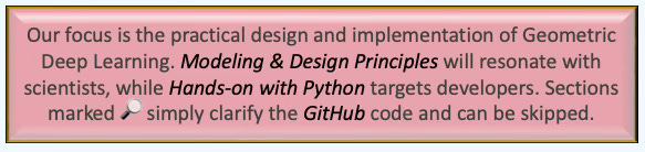
🎨 Modeling & Design Principles

Overview

The first article [ref 1] introduced the Fisher (Riemannian) metric for four basic distributions—Exponential, Geometric, Poisson, and Binomial—and demonstrated its use in computing the exponential and logarithm maps.
This follow-up explores core geometric concepts in greater depth, including the Fisher-Rao distance between distribution parameters and the inner product of vectors in the tangent space

Fisher Metric

A Fisher-Riemann manifold is a differentiable manifold MM whose points correspond to probability distributions p(x∣θ) from a statistical model parameterized by θ∈Θ⊂Rn, and which is equipped with the Riemannian metric g [ref 2]

\( g_{j k}(\theta)=\int_X \frac{\partial \log p(x, \theta)} {\partial \theta_j}\frac{\partial \log p(x, \theta)} {\partial \theta_k} p(x, \theta) d x \)

The Fisher information metric for a continuous probability density function p is defined (outer product formulation).

\(I_{X}(\theta)=g(\theta)= \int_{X}^{.} \left( \frac{\partial \ log \ p(x|\theta)}{\partial \theta} \right)^2.p_{\theta}(x).dx\)

Given that the expectation and differentiator operators can be interchanged. the metric can also be computed as (Hessian formulation)

\(I_{X}(\theta)=- \int_{X}^{.} \frac{\partial^2 log \ p(x|\theta)}{\partial \theta^2}.p_{\theta}(x).dx \ \ \ [A]\)

📌 Although not a strict rule, data scientists favor the the outer product formulation for the Fisher-Rao metric while the Hessian formulation is most commonly used by mathematicians.

The Fisher information induces a positive semi-definite metric on the parameter manifold, allowing the use of tools from differential/Riemannian geometry

The Fisher metric is invariant under sufficient statistics, making it intrinsic to the statistical model.

Fisher-Riemann manifolds are Riemannian manifolds whose metric is derived from the Fisher information metric—a central concept in information geometry. They arise naturally when treating families of probability distributions as smooth geometric objects [ref 3].

⚠️ The terminology found in the literature can be confusing. Strictly speaking the Fisher-Riemann manifold is the manifold of distributions equipped with the Fisher-Rao metric. It is also called the Fisher information manifold or the statistical manifold.

Fisher-Rao Distance

The Fisher–Rao distance quantifies the dissimilarity between two probability distributions on a statistical manifold equipped with the Fisher information metric. It represents the length of the shortest path (geodesic) connecting two points (distributions) θ1 and θ2 on this manifold.

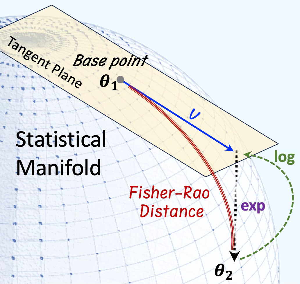
Fig. 1 Visualization of the Fisher-Rao distance (Geodesic) of a statistical manifold

Given γ(t) a smooth curve parameterized with t, the distance between θ1 and θ2 on a statistical manifold is defined as:

\(\begin{matrix} \gamma(0)=\theta_{1}, \gamma(1)=\theta_{2} \\ d_{FR}(\theta_{1}, \theta_{2}) = \underset{\gamma}{inf}\int_{0}^{1}\sqrt{\frac{\mathrm{d} \gamma}{\mathrm{d} t}^Tg_{ij}\frac{\mathrm{d} \gamma}{\mathrm{d} t}}dt \end{matrix}\)

This formulation captures the intrinsic geometry of the statistical manifold, with the Fisher information matrix acting as the Riemannian metric tensor.

📌 Computing the Fisher–Rao distance involves solving the geodesic equations derived from the Fisher information metric. However, some closed-form distributions have explicit expressions. This article illustrates the Fisher information matrix with single parameter distributions.

Inner Product of Vectors/Parameters

This inner product measures the infinitesimal change in the log-likelihood function, capturing the sensitivity of the probability distribution to changes in the parameters.

Given two vectors u and v at a point θ on a statistical manifold defined as

\(\overrightarrow{u} =\sum_{i=1}^{d}u^{i}\frac{\partial }{\partial \theta}, \ \ \ \overrightarrow{v} =\sum_{i=1}^{d}v^{i}\frac{\partial }{\partial \theta}\)

The inner product of under the Fisher-Rao metric at a point θ on a statistical manifold is computed as

\(\left< \overrightarrow{u},\overrightarrow{v} \right>_{\theta}=\sum_{i,j=1}^{d} g_{ij}(\theta)u^{i}v^{j} \ \ \ \ \ [C]\)

The norm is easily computed as

\(\left\| \overrightarrow{u}\right\|_{\theta}=\sqrt{<\overrightarrow{u},\overrightarrow{u}>_{\theta}}=\sqrt{\sum_{i,j=1}^{d} g_{ij}(\theta)u^{i}u^{j}} \ \ \ \ \ \ [D]\)

📌 We use the covariant indexes for the Fisher metric and contra-variant indexes for the vector coordinates.

Closed-form distributions

Exponential Distributions

Given a rate parameter θ > 0 the probability density function of the exponential distribution is

\(p(x|\theta)= \begin{matrix} \theta e^{-\theta x} & x > 0 \\ 0 \ \ \ \ \ \ \ & x \leq 0 \end{matrix} \)

with the Fisher-Rao metric g computed as

\(g(\theta )= \frac{1}{\theta^{2}}\)

The formula for the distance between θ1 and θ2 is

\(d_{FR}(\theta_{1}, \theta_{2})=2\left |log\left ( \frac{\theta_{2}}{\theta_{1}} \right ) \right | \ \ \ \ \ [1]\)

The inner product of two vectors u, v at parameter θ is computed as

\(\left< \overrightarrow{u},\overrightarrow{v}\right>_{\theta}=\frac{\overrightarrow{u}\overrightarrow{v}}{\theta^2} \ \ \ \ \ [2]\)

Geometric Distributions

Given the probability of success p at each trial, the probability of success after k trials is defined as

\( p(X=k)=p(1-p)^{k} \)

with the Riemannian metric g

\(g(p)=\frac{1}{p^{2}}+\frac{1}{(1-p)^{2}} \)

and the distance between two point p1 and p2 on the Geometric manifold is

\(d_{FR}(p_{1},p_{2})=\left | \int_{p_{1}}^{p_{2}} \sqrt{ \frac{1}{p^{2}}+\frac{1}{(1-p)^{2}}} dp\right | \ \ \ \ \ \ [3]\)

The inner product of two vector u, v at point p is computed as

\(\left< \overrightarrow{u},\overrightarrow{v}\right>_{p}=\left ( \frac{1}{p^2}+ \frac{1}{(1-p)^2}\right )\overrightarrow{u}.\overrightarrow{v} \ \ \ \ \ [4]\)

Poisson Distributions

Given a Poisson distribution with the expectation λ (rate parameter) events for a specific interval, the probability of k events in the same interval is

\(p(x=k|\lambda)=\frac{e^{-\lambda}\lambda^{k}}{k!} \ \ \ \ \ k \in \left\{0, 1, 2, .., \lambda \right\}\)

with the Fisher metric g defined as

\(g(\lambda)=\frac{1}{\lambda}\)

and the distance between two parameters λ1 and λ2

\(d_{FR}(\lambda_{1}, \lambda_{2})=2 \left | \sqrt{\lambda{2}}-\sqrt{\lambda{1}} \right | \ \ \ \ \ \ \ [5]\)

The inner product of two vector u, v at point λ is computed as

\(\left< \overrightarrow{u}, \overrightarrow{v}\right>_{\lambda}=\frac{\overrightarrow{u}\overrightarrow{v}}{\lambda} \ \ \ \ \ \ [6]\)

Binomial Distributions

Binomial Distribution has a closed form in the case number of draws is fixed. Given a probability distribution of success p in a sequence of n independent experiments (or number of draws).

\(p(X=k)=\binom{n}{k}p^{k}(1-p)^{n-k} \ \ \ \ k={0, 1, ... n} \ \ \ \ n \ constant \)

with the Fisher metric g:

\(g(p)=\frac{n}{p(1-p)} \ \ \ \ \ n \ constant \)

The distance between two points p1 and p2 on the Binomial manifold given a fixed number of experiments n

\(2\sqrt{n}\left | arcsin(\sqrt{p_1})- arcsin(\sqrt{p_2})\right | \ \ \ \ \ [7]\)

📌 Many complex, high-dimensional statistical manifolds—particularly multivariate ones—lack closed-form expressions for fundamental geometric components like the Fisher metric, exponential map, or geodesic paths.
In such cases, practitioners must resort to numerical techniques, including finite-difference ODE solvers (e.g., Runge–Kutta), geodesic shooting or path-based solvers, and various interpolation methods to approximate these quantities faithfully.

⚙️ Hands-on with Python

Environment

Libraries: Python 3.12.5, PyTorch 2.5.0, Numpy 2.2.0, Geomstats 2.8.0
Source code is available at Github.com/patnicolas/geometriclearning/informationgeometry/fisher_rao
To enhance the readability of the algorithm implementations, we have omitted non-essential code elements like error checking, comments, exceptions, validation of class and method arguments, scoping qualifiers, and import statements.

Setup

We leverage the implementation of the statistical manifold by subclassing CFStatisticalManifold [ref 1]. This implementation relies on the Geomstats library to generate the random point for each of the statistical manifolds [ref 4 & 5].

⚠️ Computing the Fisher metric in Geomstats requires either the Autograd or PyTorch backend. This is simply accomplished by setting the environment variable GEOMSTATS_BACKEND.

The constructor takes the following arguments

The statistical manifold, info_manifold.
Upper and lower bounds of the interval for the random variable.

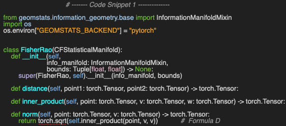
The norm (Equation D) is computed directly from the inner product of a vector by itself.

📈 Evaluation

Let’s implement the analytics formula to compute the distance for each of the statistical manifolds as a direct application of the formulas described in the previous section.

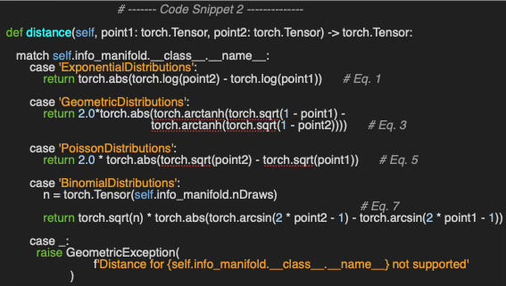
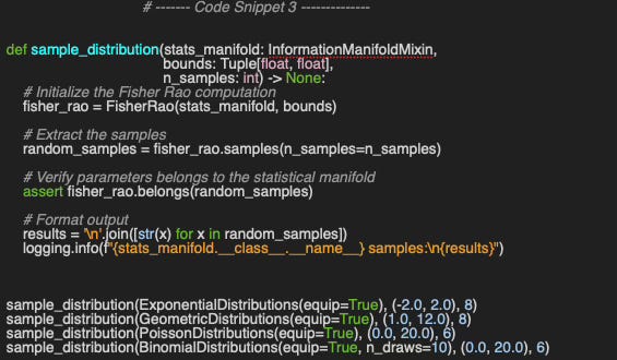
The first step is to generate n_samples random points on the statistical manifold, stats_manifold for the 4 univariate distributions with the relevant interval bounds (Code snippet 3)

Output:

ExponentialDistributions samples:
0.2551, 0.3307, 0.6764, 0.6447, 0.1431, 0.4753, 0.2847, 0.8912

GeometricDistributions samples:
0.1476, 0.4375, 0.5165, 0.5825, 0.1973, 0.6029, 0.5535, 0.2298

PoissonDistributions samples:
18.2592, 1.5876, 19.5412, 14.2694, 10.6064, 15.5452

BinomialDistributions samples:
0.6866, 0.7174, 0.3928, 0.5364, 0.1098, 0.1504

Next we evaluate the distance of two random points of each of the 4 statistical manifolds (Code snippet 4).

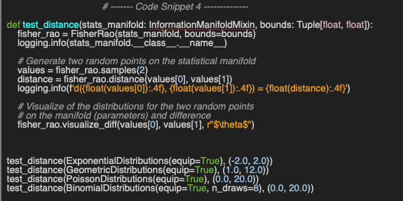
Output

ExponentialDistributions  d(0.8440, 0.8492) = 0.0062
GeometricDistributions    d(0.0131, 0.4401) = 0.0487
PoissonDistributions      d(18.5083, 11.2240) = 1.9038
BinomialDistributions     d(0.6957, 0.4829) = 1.2344

We visualize the probability density function for these 2 randomly generated points (single parameters) for each of the 4 statistical manifolds.

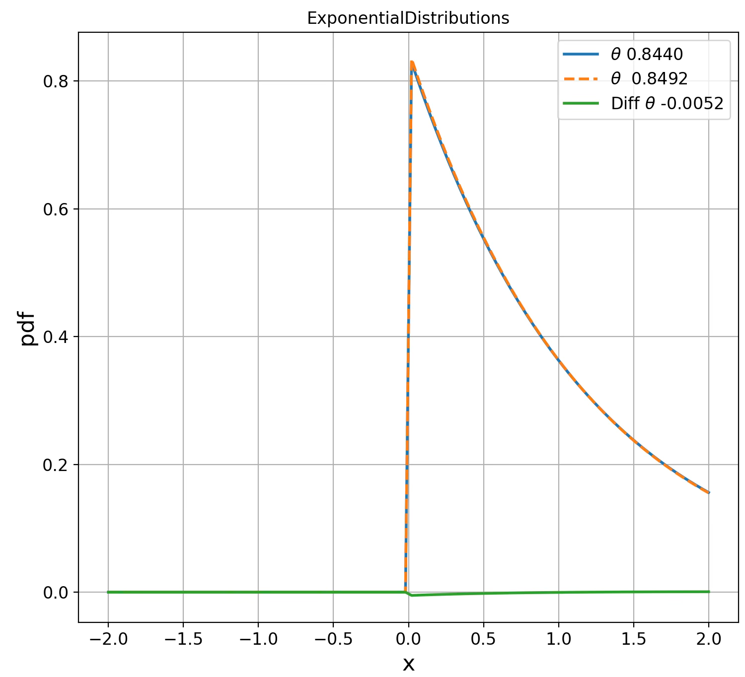
Fig. 2 Visualization of Exponential distribution for two points on Fisher manifolds

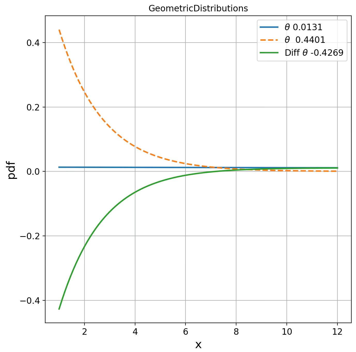
Fig. 3 Visualization of Geometric distribution for two points/parameters on Fisher manifolds

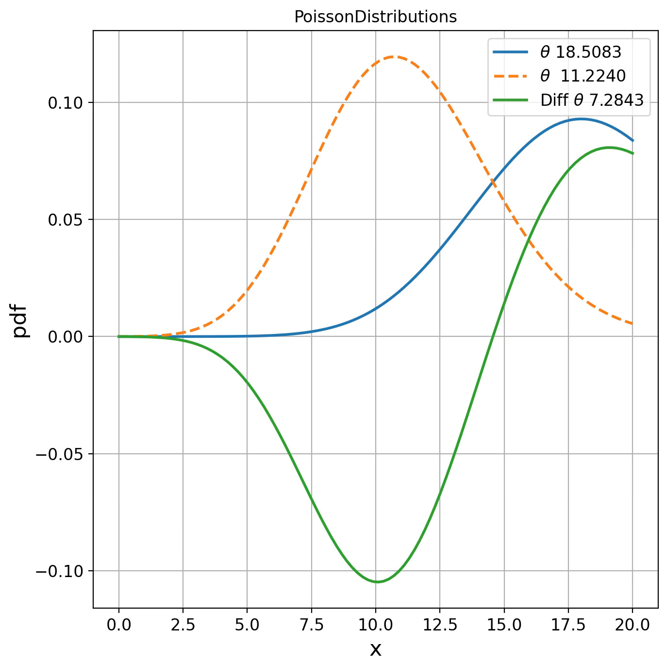
Fig. 4 Visualization of Poisson distribution for two points on Fisher manifolds

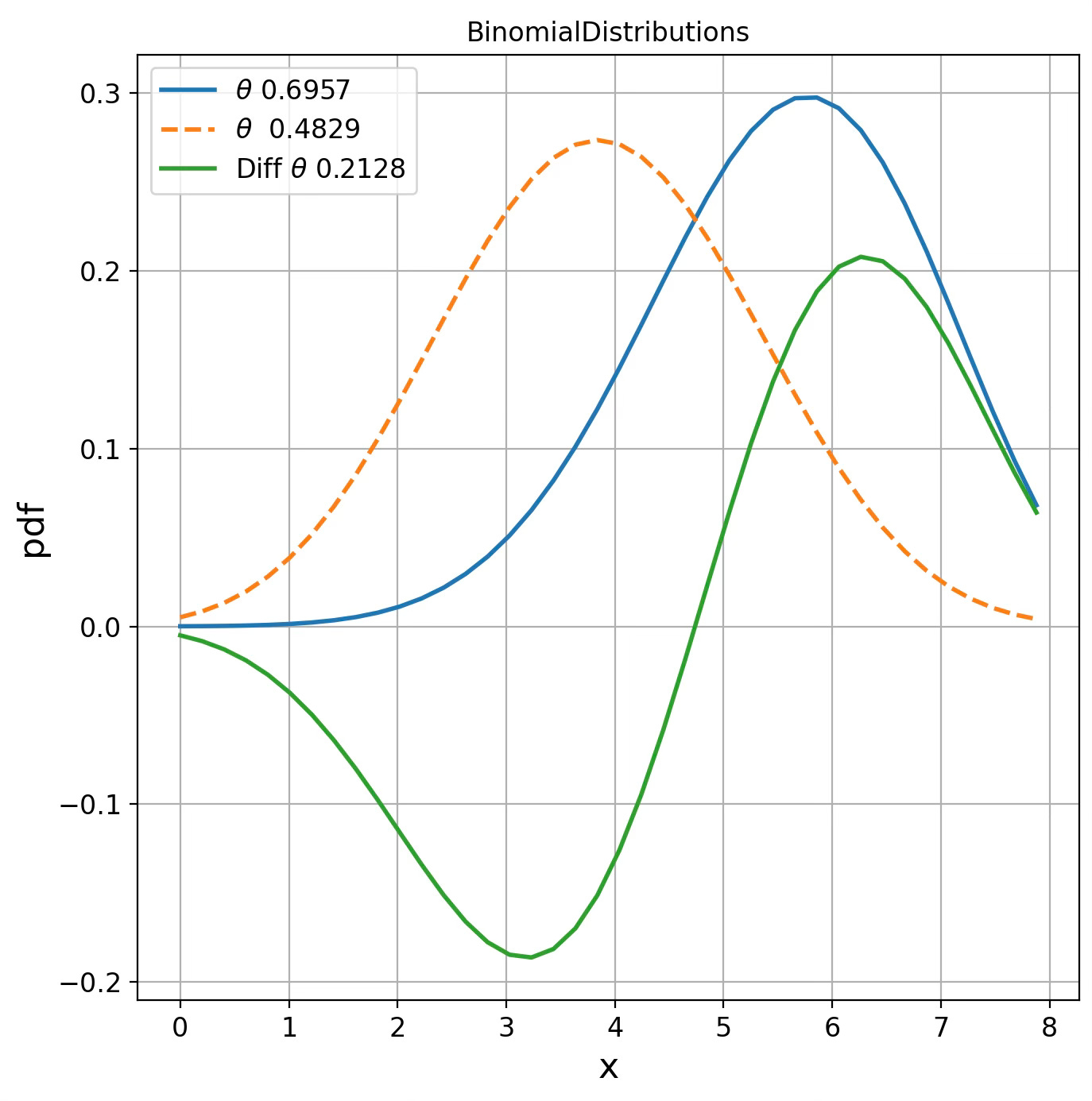
Fig. 5 Visualization of Binomial distribution for two points on Fisher manifolds

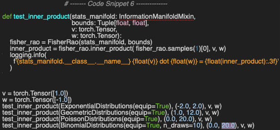
Implementing the inner product between two vectors, v and w, at a given point on each of the four statistical manifolds is a straightforward application of the formula introduced in the previous section (Code snippet 4).

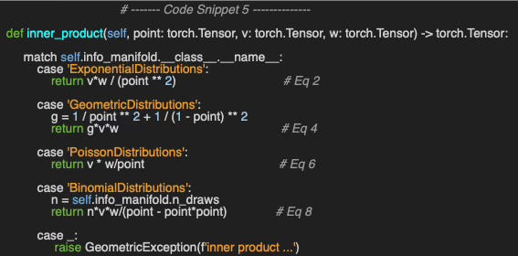
Let’s compute the inner product of two vectors/parameters u, v as follows

u=1.0, v=-1.0
u=1.0, v=0.0
u=2.0, v=0.5

Output

ExponentialDistributions 1.0 dot -1.0 = -3.600
GeometricDistributions   1.0 dot -1.0 = -8.240
PoissonDistributions     1.0 dot -1.0 = -0.157
BinomialDistributions    1.0 dot -1.0 = -221.076

ExponentialDistributions 1.0 dot 0.0 = 0.000
GeometricDistributions   1.0 dot 0.0 = 0.000
PoissonDistributions     1.0 dot 0.0 = 0.000
BinomialDistributions    1.0 dot 0.0 = 0.000

ExponentialDistributions 2.0 dot 0.5 = 1.180
GeometricDistributions   2.0 dot 0.5 = 78.837
PoissonDistributions     2.0 dot 0.5 = 0.128
BinomialDistributions    2.0 dot 0.5 = 42.672

As expected, the inner product of the vectors +1.0 and –1.0 is negative, while that of +1.0 and 0.0 is 0.0.

Finally, we proceed to compute the norms of vectors on the four different statistical manifolds.

ExponentialDistributions Norm(0.5) = 1.186
GeometricDistributions Norm(0.5) = 1.468
PoissonDistributions Norm(0.5) = 0.182
BinomialDistributions Norm(0.5) = 3.898

ExponentialDistributions Norm(1.0) = 1.398
GeometricDistributions Norm(1.0) = 2.893
PoissonDistributions Norm(1.0) = 0.385
BinomialDistributions Norm(1.0) = 16.802

The value of the norm reflects the curvature at a given point. of the manifold.

🧠 Key Takeaways

✅ We delve deeper into closed-form statistical manifolds by examining both the Fisher–Rao distance and the inner product on their tangent spaces.

✅ Using PyTorch, we directly implement the Fisher information metric, compute distances, and evaluate tangent-space inner products for the exponential, Poisson, geometric, and binomial distributions.

✅ For generating sample points on these manifolds, we leverage Geomstats for convenience and consistency

📘 References

🛠️ Exercises

Q1: What are the most commonly used numerical integration techniques to compute exponential or logarithm maps of complex statistical manifolds without closed-form?
Q2: Can you write the steps to the Fisher metric formula for the exponential distribution?
Q3: Given the Fisher metric for the Poisson distribution, can you generate the distance between two points on the manifold?

👉 Answers

💬 News & Reviews

This section focuses on news and reviews of papers pertaining to geometric deep learning and its related disciplines.

Paper Review: Analysis of Static & Dynamic Batching Algorithms for Graph Neural Networks D. Speckhard, T, Bechtel, S. Kehl, J. Godwin, C Draxl

Graph Neural Networks (GNNs) are computationally expensive to train, making them strong candidates for batching techniques commonly used in standard deep learning models. This paper evaluates two batching strategies—static and dynamic.

Libraries such as JGraph (JAX-based) and PyTorch Geometric support dynamic batching, while TensorFlow offers both static and dynamic batching.

Dynamic Batching

Implementation varies across libraries but follows a common approach:

Estimate padding constraints for each batch (size is a multiple of 64) by sampling a subset of the dataset.
Iteratively add graphs to the batch until the padding limit is reached.

Static Batching

This method adds a fixed number of graphs per batch and then pads them to a predefined size.

A common trick is to introduce dummy graphs so that the total number of nodes and edges is a power of 2, optimizing memory utilization.

Experimental Setup

Environment: 4x A100 GPU with NVLINK using:
Datasets: QM9 (chemical properties) & AFLOW (material properties)
Models: SchNet (Graph Convolutional Network) & MPEU (Message-Passing Neural Network)

Key Findings

Dynamic batching is slower than static batching due to the overhead of managing varying padding constraints.
Static batching techniques, particularly, batching with total nodes and edges as multiples of 64 and batching with totals as powers of 2n achieved the lowest average training times.
Dataset characteristics and batch size tuning can improve performance by over 33%.

Patrick Nicolas has over 25 years of experience in software and data engineering, architecture design and end-to-end deployment and support with extensive knowledge in machine learning.
He has been director of data engineering at Aideo Technologies since 2017 and he is the author of "Scala for Machine Learning", Packt Publishing ISBN 978-1-78712-238-3 and Geometric Learning in Python Newsletter on LinkedIn.