

Neighbors Matter: How Homophily Shapes Graph Neural Networks
Expertise Level ⭐⭐

Given the wide range of configuration choices, setting up a Graph Neural Network can be daunting. Wouldn’t it be helpful to have a criterion that at least filters out less promising architectures?
Node and edge homophily ratios might offer just that guidance.
👉 The animation above is implemented by the method play_animation in geometriclearning/play/graph_homophily_play.py

🎯 Why this matters
Purpose: Imagine being able to analyze a dataset upfront to determine the optimal configuration for a Graph Neural Network. Homophily provides a principled way to assess whether proximity in the graph structure—through nodes or edges—correlates with similarity in labels or classes.
Audience: Data scientists and engineers designing, training and validating graph neural networks
Value: Learn to compute graph homophily and use it to guide the design of your Graph Neural Network.
🎨 Modeling & Design Principles
⚠️ I strongly recommend to review my articles introducing PyTorch Geometric Taming PyTorch Geometric for Graph Neural Networks and Graph loaders Demystifying Graph Sampling & Walk Methods
What is Homophily
In Graph Neural Networks (GNNs), homophily measures the tendency of nodes with the same label (or similar features) to be connected.
High homophily graphs (e.g., citation networks) have neighbors likely sharing labels, while low homophily graphs (e.g., Amazon co-purchase graphs) might not.
The homophily of a graph characterizes how likely nodes with the same label are near each other in a graph.
Let’s start with the mathematical definition. Let G=(V,E) be a graph with a set of nodes (vertices) V, a set of edges E, label yv of node v and a neighbors of node v, N(v)., there are 3 types of homophily ratios:
Node homophily ratio: Average fraction of same-label neighbors per node.
Edge homophily ratio: The fraction of edges in a graph which connects nodes that have the same class label.
Class insensitive edge homophily ratio: Edge homophily is modified to be insensitive to the number of classes and size of each class. C number of classes, |Ck| number of nodes of class k and hk denotes the edge homophily ratio of class k.
In a nutshell, Edge homophily answers: "How likely is it that a random edge connects same-label nodes?" while Node homophily answers: "How homophilic is the neighborhood of a typical node?.
⚠️ Several factors can explain the discrepancy between node homophily and edge homophily ratios, including:
Edge homophily tends to be biased toward high-degree nodes, whereas node homophily gives equal weight to all nodes.
If a particular class consists primarily of high-degree nodes, it can artificially inflate the edge homophily due to class imbalance.
Node homophily typically excludes isolated nodes, which can further contribute to the difference.
Why Homophily
Homophily is a key property of Graph Neural Networks that helps controlling:
Architecture decision
Depth of models
Aggregation method
Training strategy
Here is a rule of thumb:
Graph with high homophily
Simple Graph Neural Network, Graph Convolutional Network or Graph Attention Networks works best
No more than two GNN layers are necessary
Graph with low homophily
Heterophily-aware Graph Neural Networks
Features transformation prior to aggregation
Residual connections
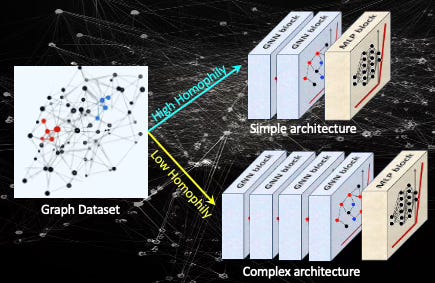
Fig. 1 Illustration of impact of Homophily on the design of a Graph Convolutional Network
In this study, we treat the distribution of node neighbor sampling as an indicator of model complexity. In the example below, the random walk used to sample neighbors of node '0' may span 1, 2, 3, or more hops.

Fig. 2 Illustration of random walk/sampling of neighboring nodes from node ‘0’
We define model complexity arbitrarily as a combination of the number of hops and the maximum number of nodes randomly selected at each hop.
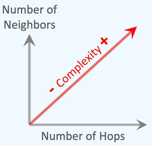
Fig. 3 Illustration of complexity of random sampling of neighboring nodes
This definition can be extended by incorporating additional factors, such as the number of Graph Convolutional layers, as illustrated earlier.
⚙️ Hands-on with Python
Environment
Libraries: Python 3.11.8, PyTorch 2.1.0, PyTorch Geometric 2.6.1, Optuna 4.2.0
Source code: geometriclearning/dataset/graph/graph_homophily.py
Evaluation: geometriclearning/play/graph_homophily_play.py
The source tree is organized as follows: features in python/, unit tests in tests/,and newsletter evaluation code in play/.
To enhance the readability of the algorithm implementations, we have omitted non-essential code elements like error checking, comments, exceptions, validation of class and method arguments, scoping qualifiers, and import statements.
Graph Convolutional Neural Networks
📌📌This section does not provide a theoretical review of Graph Neural Networks (GNNs). Instead, there are numerous high-quality tutorials and detailed explanations available in both printed resources and online materials. I recommend the following references 1, 2, 3, & 4 as tutorial..
Overview
A Graph Neural Network (GNN) is an optimizable transformation on all attributes of the graph (nodes, edges, global context) that preserves graph symmetries (permutation invariances). GNN takes a graph as input and generate/predict a graph as output.
Data on manifolds can often be represented as a graph, where the manifold's local structure is approximated by connections between nearby points. GNNs and their variants (like Graph Convolutional Networks (GCNs) extend neural networks to process data on non-Euclidean domains by leveraging the graph structure, which may approximate the underlying manifold.
Our Evaluation Model
For our study we use a Graph Convolutional Neural Network defined in a previous article, How to Tune a Graph Neural Networks - Hyperparameters Tuning Framework with the following configuration:
2 Graph Convolutional blocks with ReLU activation and no pooling
1 fully connected output block with LogSoftmax activation.
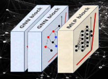
Fig. 4 Illustration of a 2 graph convolutional layer model used in this study
We apply the neighbor node sampling method, described in Demystifying Graph Sampling & Walk Methods - Neighbor Node Sampling to embed and aggregate node attributes from neighboring nodes with the following configuration:
{
   'id': 'NeighborLoader',
   'num_neighbors': [12, 6, 3],
   'batch_size': 64,
   'replace': True,
   'num_workers': 4
}
Datasets
PyTorch Geometric (PyG) offers a comprehensive collection of graph datasets across various domains [ref 5 & 6]. These graph datasets are accessible through dedicated class in the torch_geometric.datasets module [ref 7].
In this study we analyze the following data sets
Cora: A standard benchmark dataset for semi-supervised node classification, containing 2,708 nodes (scientific publications) and 5,429 edges (citations). Each node is described by a 1,433-dimensional feature vector. This dataset is also included in torch_geometric.datasets.Planetoid class collection.
CiteSeer: A citation network containing 3,312 scientific publications classified into six categories. The network contains 4,715 edges, with each node represented by a very large 3,703-dimensional feature vector. This dataset is also included in torch_geometric.datasets.Planetoid class collection.
PubMed: Consists of 19,717 scientific publications from the PubMed database, each pertaining to diabetes and classified into one of three classes. The citation network includes 44,338 edges, and each node has a 500-dimensional feature vector. This dataset is also included in torch_geometric.datasets.Planetoid class collection.
Wikipedia: contains 11,701 nodes, 216,123 edges, 10 classes and 20 different training splits.
Flickr: Contains descriptions and common properties of 89,250 images along with 899.756 edges and a 500-dimensional feature vector. It is defined in torch_geometric.datasets.Flickr class.
🔎 Node & Edge Homophily
⏭️ This section guides you through the design and code.
We begin by defining an enumeration, GraphHomophilyType, to represent the four categories of homophily ratios described earlier.
The GraphHomophily class, shown in code snippet 1, encapsulates the computation of node homophily, edge homophily, and class-insensitive edge homophily. It provides two constructors:
__init__: The default constructor, which initializes the class with a given graph data and the selected type of homophily computation.
build: An alternative constructor that creates an instance using a predefined PyTorch Geometric dataset along with the specified homophily computation type.
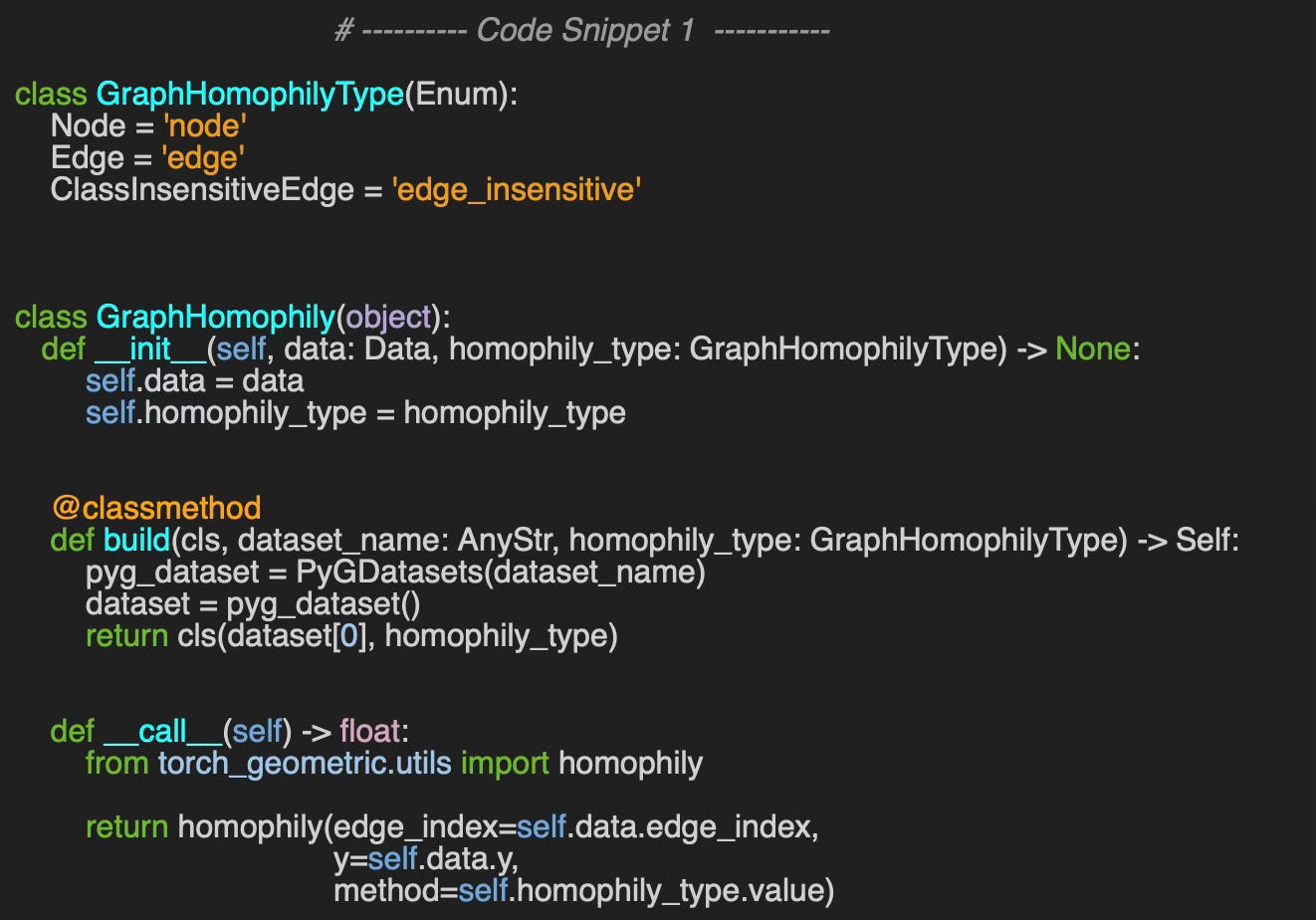
The actual computation is performed in the __call__ dunda method which invokes the PyTorch Geometric homophily function
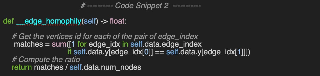
We include a homegrown implementation of the computation of the edge homophily (Code snippet 2) for reference.
We compute the various homophily ratios for the 5 PyTorch Geometric datasets: Cora, PubMed, CiteSeer, Wikipedia and Flickr (Code snippet 3).
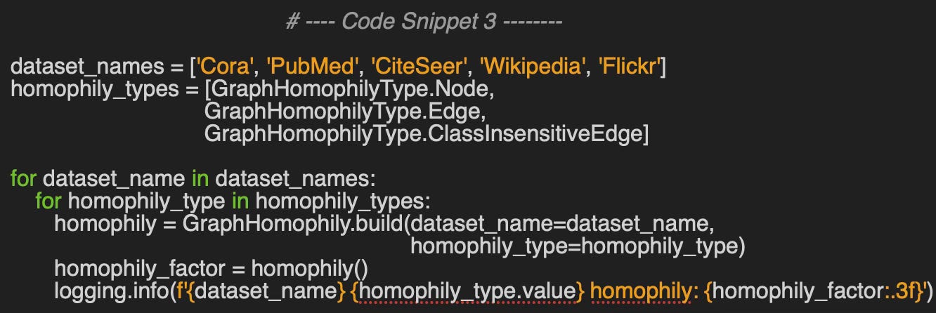
👉 Source code for test is available at geometriclearning/play/graph_homophily_play.py
Cora node homophily: 0.825
Cora edge homophily: 0.810
Cora edge_insensitive homophily: 0.766
PubMed node homophily: 0.792
PubMed edge homophily: 0.802
PubMed edge_insensitive homophily: 0.664
CiteSeer node homophily: 0.706
CiteSeer edge homophily: 0.736
CiteSeer edge_insensitive homophily: 0.627
Wikipedia node homophily: 0.104
Wikipedia edge homophily: 0.235
Wikipedia edge_insensitive homophily: 0.059
Flickr node homophily: 0.322
Flickr edge homophily: 0.319
Flickr edge_insensitive homophily: 0.070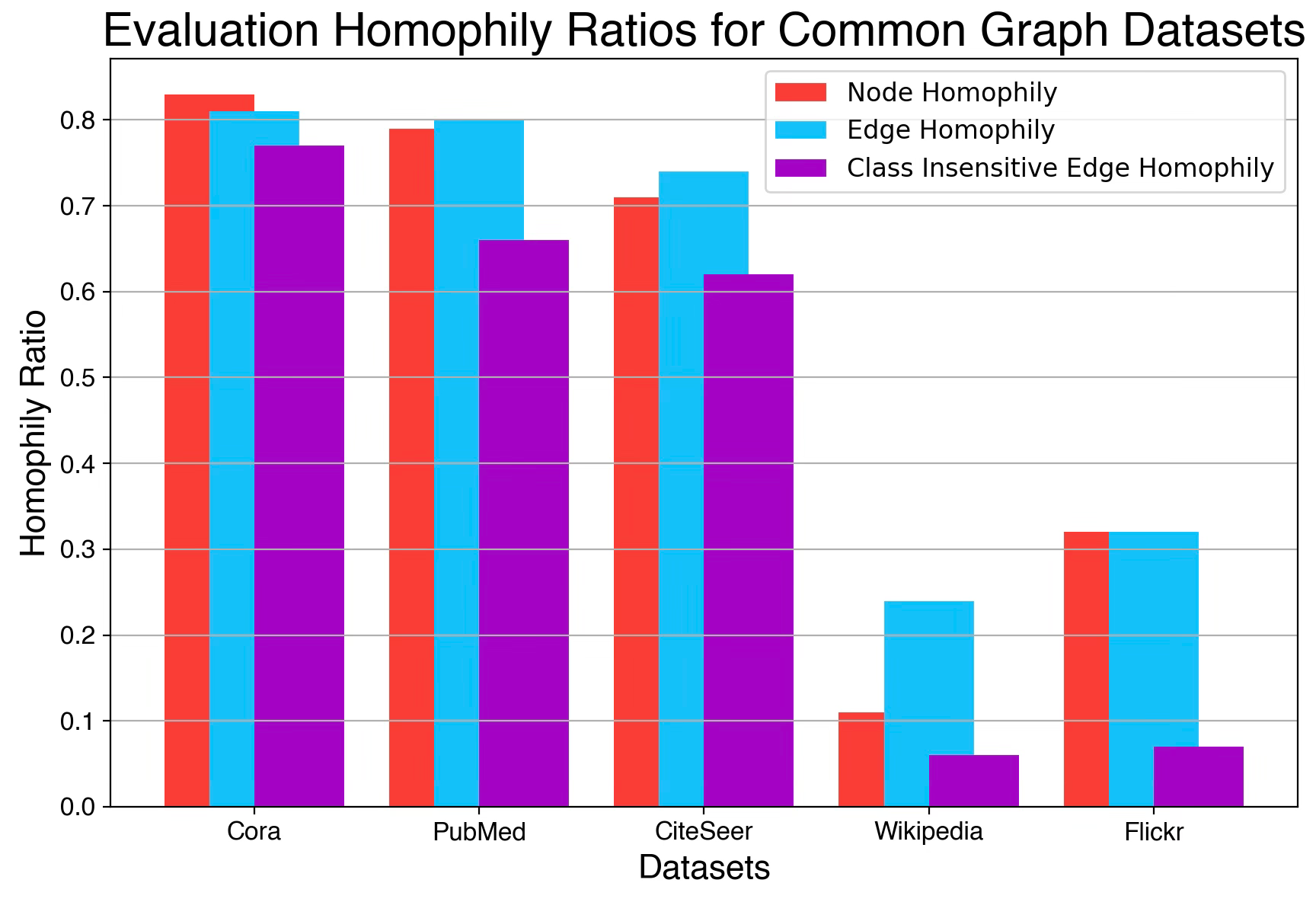
Fig. 5 Bar Chart for Node, Edge and Class Insensitive Edge Homophily for 5 PyTorchGeometric Datasets
We use Cora as a representative high-homophily dataset and Flickr to illustrate a low-homophily scenario.
Training & Validation
The training and validation of our model are described in details in Plug & Play Training of Graph Neural Networks
As a reminder we used the following hyperparameters
{
    'dataset_name': 'Flickr',
        # Model training Hyperparameters
    'learning_rate': 0.0005,
    'momentum': 0.90,
    'batch_size': nn.NLLLoss(),
    'loss_function': None,
    'encoding_len': 7,
    'train_eval_ratio': 0.9,
    'epochs': 20,
    'weight_initialization': 'xavier',
    'optim_label': 'adam',
    'drop_out': 0.25,
    'is_class_imbalance': True,
    'class_weights': torch.Tensor([0.1853, 0.1127, 0.1539, 0.2003,
                          0.0423, 0.2796, 0.0259])
    'patience': 2,
    'min_diff_loss': 0.02,
        # Performance metric definition
    'metrics_list': ['Accuracy', 'Precision', 'Recall', 'F1'],
        # ...
}
The validation records and display the 4 metrics (Accuracy, Precision, Recall, F1), training and validation loss for various Node Neighbor Sampling distributions:
Single hop - 4 neighbors [4]
Two hops - First: 4 neighbors, Second: 2 neighbors [10, 4]
Three hops - First: 12 neighbors, Second: 6 neighbors, Third: 3 neighbors [12, 6, 3]
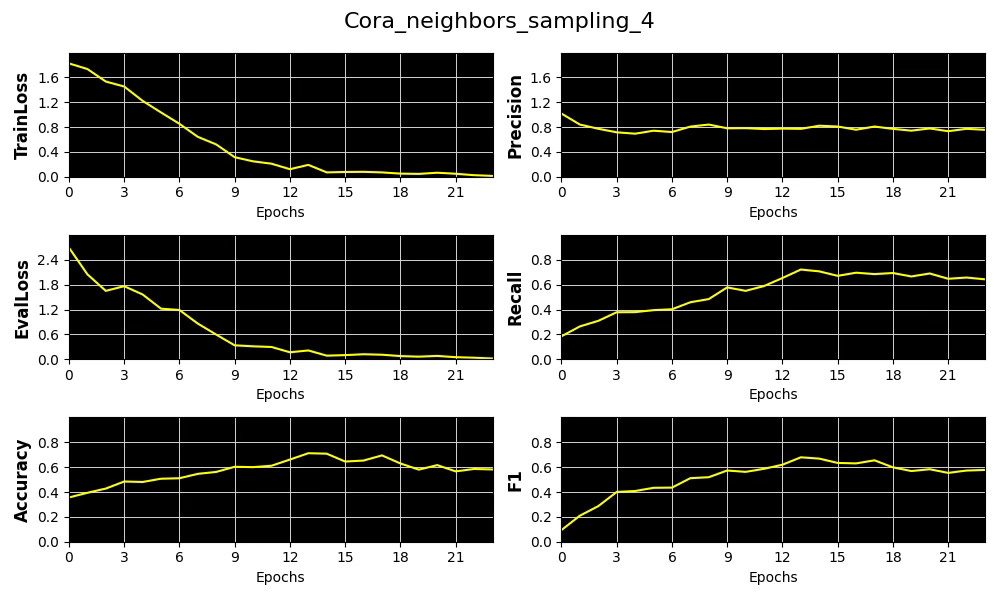
Fig. 6 Plots of metrics, training & validation loss for the distribution of number of sampled neighboring nodes [4] for Cora dataset
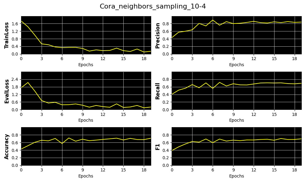
Fig. 7 Plots metrics, training & validation loss for the distribution of number of sampled neighboring nodes [10, 4] for Cora dataset
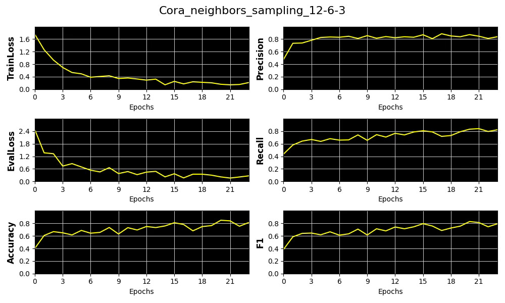
Fig. 8 Plots of metrics, training & validation loss for the distribution of number of sampled neighboring nodes [12, 6, 3] for Cora dataset
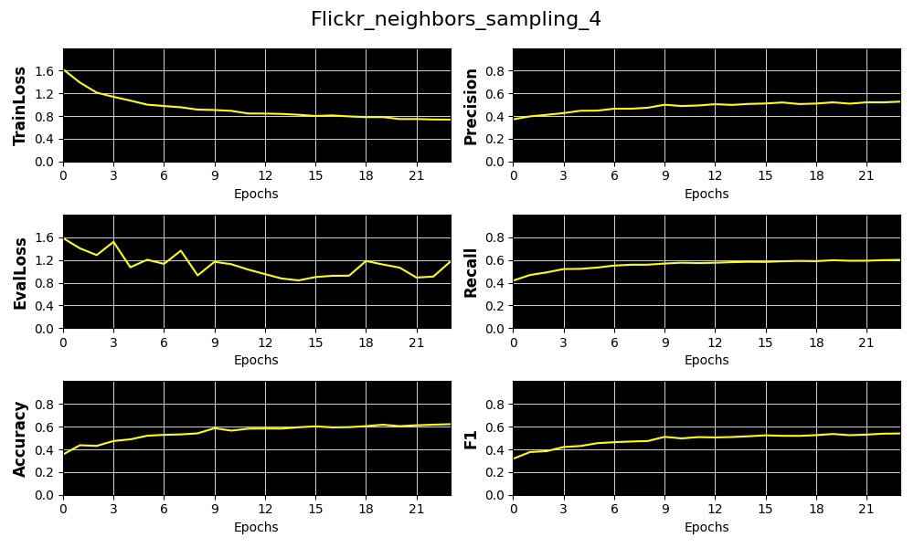
Fig. 9 Plots of metrics, training & validation loss for the distribution of number of sampled neighboring nodes [4] for Flickr dataset
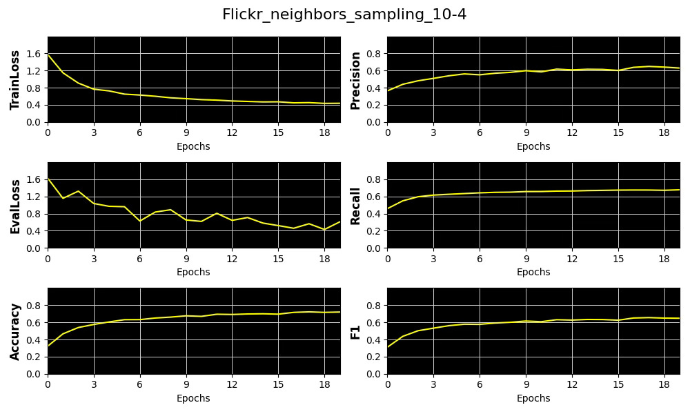
Fig. 10 Plots of 4 key metrics, training & validation loss for the distribution of number of sampled neighboring nodes [10, 4] for Flickr dataset
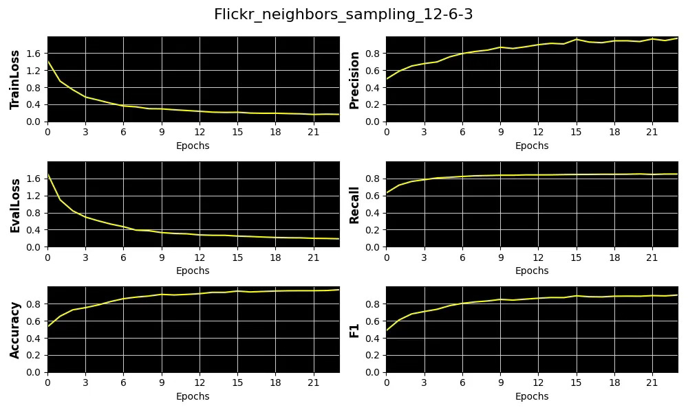
Fig. 11 Plots of 4 key metrics, training & validation loss for the distribution of number of sampled neighboring nodes [12, 6, 3] for Flickr dataset
📈 Analysis
Setup
We select precision as our primary performance metric that we plot against the average of Node and Edge Homophily ratios for each of the 3 node neighbor sampling configuration for Cora and Flickr datasets.
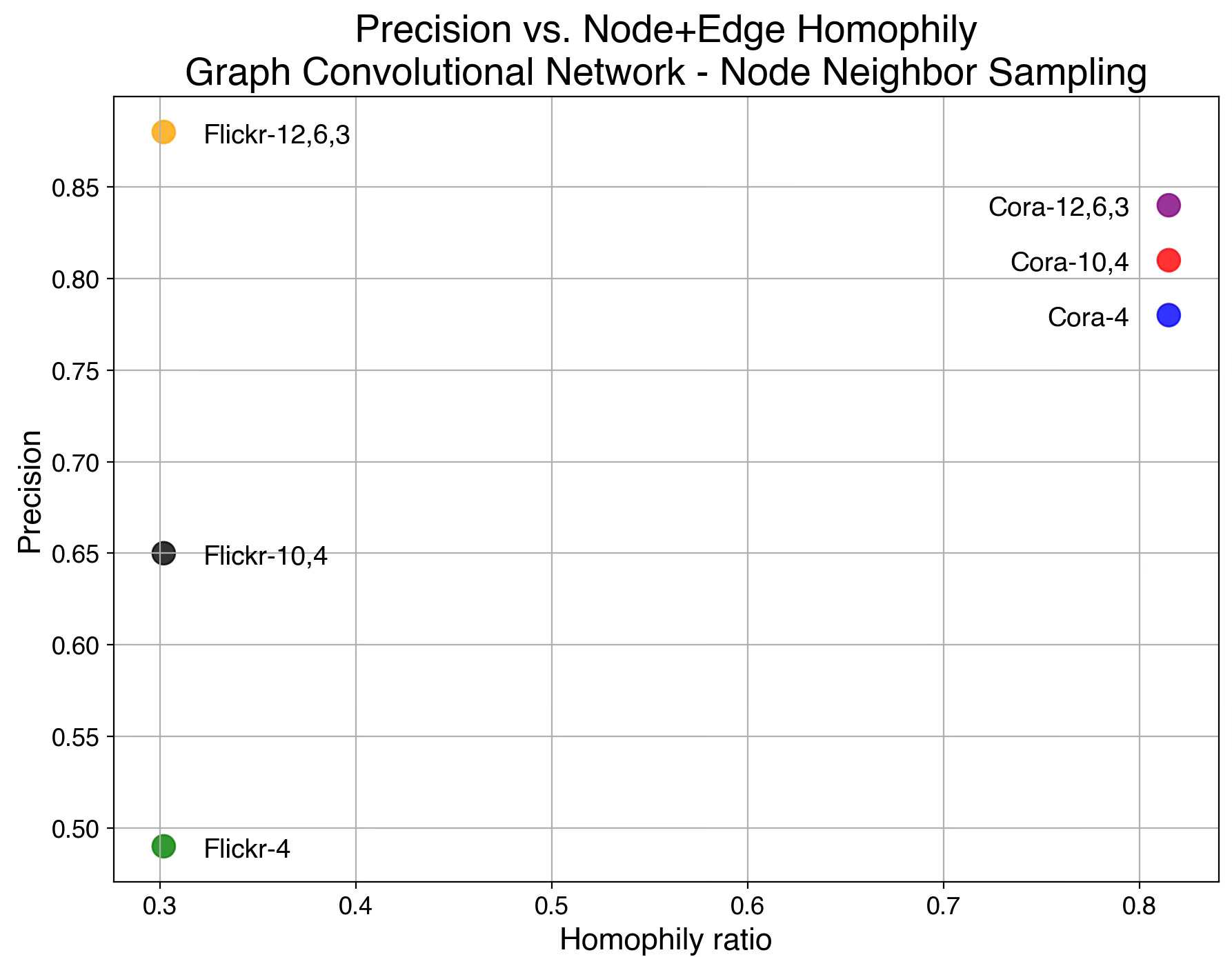
Fig. 12 Scatter plot of precision vs. average (node, edge homophily) for Cora and Flickr data sets with 3 configuration of node neighbors sampling
Conclusion
The results show that increasing the complexity of our model—specifically through Node Neighbor Sampling distribution—enhances precision on the low-homophily dataset (Flickr), while having minimal effect on the high-homophily dataset (Cora).
🧠 Key Takeaways
✅ Graph homophily refers to the tendency of connected nodes to share similar labels or attributes.
✅ Node and edge homophily can serve as useful indicators of the structural complexity required for a Graph Neural Network.
✅ While a simple two-layer Graph Convolutional Network may suffice for datasets with high homophily, lower homophily—or heterophily—typically demands more sophisticated architectures.
✅ We demonstrated how homophily affects node classification precision in a GCN by using the distribution of sampled neighbors as a proxy for model complexity.
📘 References
A Practical Tutorial on Graph Neural Networks I. Ward, J. Joyner, C. Lickfold, Y. Guo, M. Bennamoun - 2012
A Comprehensive Introduction to Graph Neural Networks - Datacamp - 2022
Graph Neural Networks: A Gentil Introduction - YouTube. A. Persson
Stanford CS: Machine Learning with Graphs - YouTube - CS-224 Stanford University Online
🛠️ Exercises
Q1: What distinguishes the node homophily ratio from the edge homophily ratio
Q2: What are the key attributes that define the complexity of a Graph Neural Network?
Q3: How can the node homophily ratio be implemented in code?
Q4: What factors contribute to the discrepancy between node and edge homophily ratios?
👉 Answers
💬 News & Reviews
This section focuses on news and reviews of papers pertaining to geometric deep learning and its related disciplines.
Paper review: Machine Learning & Algebraic Geometry Vahid Shahverdi 2023
This concise presentation synthesizes and summarizes various research findings at the crossroads of machine learning and algebraic geometry. The author begins by reviewing essential aspects of machine learning, including Kernel methods, feedforward neural networks, and the universal approximation theorem.
Algebraic geometry's application to machine learning
The paper explores how activation functions correlate with the mathematical structure involved in minimizing the loss function under three scenarios:
Linear Neural Networks
Neural Networks employing polynomial approximations for activation.
Networks utilizing ReLU activation.
It defines the space of neural network weights as a low-dimensional manifold, where the loss function's minimization occurs across the weights on this manifold.
Applying machine learning to algebraic geometry
The goal is to comprehend the topology of hypersurfaces using machine learning techniques. Here, a neural network delineates the boundary decision among regions or chambers within hypersurfaces.
Note: The reader would benefit from basic knowledge in algebraic topology and geometry
Expertise Level
⭐ Beginner: Getting started - no knowledge of the topic
⭐⭐ Novice: Foundational concepts - basic familiarity with the topic
⭐⭐⭐ Intermediate: Hands-on understanding - Prior exposure, ready to dive into core methods
⭐⭐⭐⭐ Advanced: Applied expertise - Research oriented, theoretical and deep application
⭐⭐⭐⭐⭐ Expert: Research , thought-leader level - formal proofs and cutting-edge methods.
Patrick Nicolas is a software and data engineering veteran with 30 years of experience in architecture, machine learning, and a focus on geometric learning. He writes and consults on Geometric Deep Learning, drawing on prior roles in both hands-on development and technical leadership. He is the author of Scala for Machine Learning (Packt, ISBN 978-1-78712-238-3) and the newsletter Geometric Learning in Python on LinkedIn.