

Plug & Play Training for Graph Convolutional Networks
Expertise Level ⭐⭐⭐

Managing, evaluating, and tuning hyperparameters and complex graph models directly in code can be both time-consuming and overwhelming. This article introduces and implements a unified JSON-based declarative interface that streamlines every stage—building, training, tuning, and testing—of a graph neural network.

🎯 Why this Matters
Purpose: Manually cataloging, updating, and tuning all possible hyper-parameters and model settings directly in code is both error-prone and time-consuming. Adopting a unified, JSON-based declarative format for all configurations can significantly streamline the process and reduce complexity
Audience: Data scientists and machine learning engineers building, training, validating and tuning graph neural networks
Value: Discover how to define and utilize a JSON-based representation of model and training parameters to design, train, and validate a graph neural network.
🎨 Modeling & Design Principles
⚠️ I strongly recommend to review my articles introducing PyTorch Geometric Taming PyTorch Geometric for Graph Neural Networks and Graph loaders Demystifying Graph Sampling & Walk Methods
Overview
Data on manifolds can often be represented as a graph, where the manifold's local structure is approximated by connections between nearby points. GNNs and their variants (like Graph Convolutional Networks - GCNs) extend neural networks to process data on non-Euclidean domains by leveraging the graph structure, which may approximate the underlying manifold. Application Social network analysis, molecular structure prediction, and 3D point cloud data can all be modeled using GNNs.
Graph Convolutional Neural Networks
Graph Neural Networks have been discussed in depth in previous articles in this newsletter [ref 1, 2]
Overview
A Graph Neural Network (GNN) is an optimizable transformation on all attributes of the graph (nodes, edges, global context) that preserves graph symmetries (permutation invariances). GNN takes a graph as input and generate/predict a graph as output.
Data on manifolds can often be represented as a graph, where the manifold's local structure is approximated by connections between nearby points. GNNs and their variants (like Graph Convolutional Networks (GCNs) extend neural networks to process data on non-Euclidean domains by leveraging the graph structure, which may approximate the underlying manifold [ref 3, 4, 5 & 6].
📌 The reminder of this paragraph is a review of topics already discussed in previous articles [ref 1, 2] that can be skipped.
Scope
There are 3 types of tasks to be performed on a GNN:
Graph-level task: Predict the property of the entire graph such as classification problems with MNIST or CIFAR images or sentiment analysis for a document or paragraph.
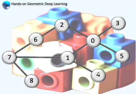
Node-level task: Predict if a node belongs to a specific class (i.e. Karate club) or image segmentation (identify the role of a pixel in an image) or part of speech a word belongs to.
Edge-level task: Predict the relationship between node (i.e. Interaction between users) that can be classified (discovery of connections between entities or nodes). The task also consists in pruning a fully connected graph into a sparse graph.
Types
Application such as social network analysis, molecular structure prediction, and 3D point cloud data can all be modeled using GNNs. Here is an overview of the major types of GNNs:
Graph Convolutional Network (GCN): GCNs generalize the concept of convolution from grids (e.g., images) to graphs. They aggregate information from a node's neighbors using normalized adjacency matrices and apply transformations to learn node embeddings.
Graph Attention Network (GAT): GATs use attention mechanisms to learn the importance of neighboring nodes dynamically. Each edge is assigned a learned weight during aggregation.
Graph Sample and Aggregate (GraphSAGE) :It learns node embeddings by sampling and aggregating features from a fixed-size neighborhood of each node, enabling scalable learning on large graphs.
Graph Isomorphism Network (GIN): GINs are designed to be as powerful as the Weisfeiler-Lehman (WL) graph isomorphism test, distinguishing graph structures more effectively.
Spectral Graph Neural Network (SGNN): SGNNs operate in the spectral domain using the graph Laplacian. They use eigenvectors of the Laplacian for convolution-like operations.
Graph Pooling Network: Graph Pooling Networks summarize graph information into a smaller representation, similar to pooling in CNNs. They can be categorized into Global and hierarchical pooling
Hyperbolic Graph Neural Network: Hyperbolic Graph Networks operate in hyperbolic space, which is well-suited for representing hierarchical or tree-like graph structures.
Dynamic Graph Neural Network: These networks are designed to handle temporal graphs, where nodes and edges evolve over time.
Relational Graph Convolutional Network (R-GCN): R-GCNs extend GCNs to handle heterogeneous graphs with different types of nodes and edges.
Graph Transformer: Graph Transformers adapt the Transformer architecture to graph-structured data using attention mechanisms and global context.
Graph Autoencoder: Graph Autoencoders are used for unsupervised learning on graphs, aiming to reconstruct graph structure and node features.
Diffusion-based GNN: As its name implies, Diffusion-based GNN uses graph diffusion processes to propagate information.
Graph Samplers
The generation of universal embeddings that apply across different applications remains a significant challenge.
PyTorch Geometric simplifies this process by encapsulating these complexities into specialized data loaders, while seamlessly integrating with PyTorch's existing deep learning modules.
PyTorch Geometric supports a large variety of graph data loader, including:
Random node loader: A data loader that randomly samples nodes from a graph and returns their induced subgraph.
Neighbor node loader: This loader partitions nodes into batches and expands the subgraph by including neighboring nodes at each step.
Neighbor link loader: This loader is similar to the neighborhood node loader except it partitions links and associated nodes into batches.
Subgraphs Cluster: Divides a graph data object into multiple subgraphs or partitions. A batch is then formed by combining a specified number of subgraphs.
Graph Sampling Based Inductive Learning Method: This is an inductive learning approach that enhances training efficiency and accuracy by constructing mini-batches through sampling subgraphs from the training graph, rather than selecting individual nodes or edges from the entire graph.
Declarative Training Configuration
The goal is to design a modular framework that streamlines the configuration of graph neural networks, sampling strategies, and hyper-parameters—enabling automated training, validation, and tuning pipeline of selected GNN models as illustrated below
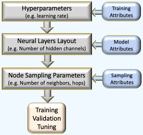
Fig. 1 Three step optimization process for architecture design, training and configuration of a Graph Neural Network.
It is critical to keep the configuration attributes for hyper-parameters, model definition and sampling method as consistent as possible. To this purpose, we select the ubiquitous JSON notation.
Adopting a declarative format to define models, hyper-parameters, and the training environment offers several advantages:
Reduces the risk of introducing new bugs
Lowers the barrier for practitioners who may not be experienced programmers
Potentially eliminates the need to retest existing implementations
Below are examples demonstrating how JSON notation can be used to configure the entire training and validation pipeline
Training environment
The following JSON descriptor defines the parameters required for training, validating and tuning your Graph Neural Model.
{
  'dataset_name': 'Sonar',
  'learning_rate': 0.0005,
  'batch_size': 64,
  'loss_function': nn.NLLLoss(weight=class_weights.to('cuda0')),
  'momentum': 0.90,
  'encoding_len': 8,
  'train_eval_ratio': 0.9,
  'weight_initialization': 'xavier',
  'optim_label': 'adam',
  'drop_out': 0.25,
  'is_class_imbalance': True,
  'class_weights': [0.25, 0.3, 0.2, 0.2, 0.05],
  'metrics_list': ['Accuracy', 'Precision', 'Recall', 'F1'],
  'plot_parameters': [
     {'title': 'Accuracy', 'x_label': 'epoch', 'y_label': 'accuracy'},
     {'title': 'Precision', 'x_label': 'epochs', 'y_label':'precision'},
     {'title': 'Recall', 'x_label': 'epochs', 'y_label': 'recall'},
     {'title': 'F1', 'x_label': 'epochs', 'y_label': 'F1'},
  ]
}
📌 We selected the parameters somewhat arbitrarily, so your list may differ slightly
Graph Convolutional Model
Neural blocks serve as the fundamental components of deep neural networks [ref 7]. A Graph Convolutional Neural Network (GCN) consists of a series of graph convolutional blocks followed by a sequence of fully connected blocks, each fully specified with an activation function, layer configuration, and optional components such as batch normalization, pooling, and dropout regularization.
{
   'model_id': 'MyModel',
   'gconv_blocks': [
      {
        'block_id': 'conv_block_1',
        'conv_layer': GraphConv(in_channels=num_node_features,
                                out_channels=hidden_channels),
        'num_channels': hidden_channels,
        'activation': nn.ReLU(),
        'batch_norm': None,
        'pooling': None,
        'dropout': 0.25
      },
      .....
   ],
   'mlp_blocks': [
      {
        'block_id': 'mlp_block',
        'in_features': hidden_channels,
        'out_features': _num_classes,
        'activation': None,
        'dropout': 0.0
      }
   ]
 }
📌 A modular description of the graph convolutional network is described in an early paragraph Graph Neural Network Components
Graph Node Sampling Method
Finally we specify the sampling method as neighbor node sampling [ref 8].
{
   'id': 'NeighborLoader',
   'num_neighbors': [12, 6, 3],
   'batch_size': 64,
   'replace': True,
   'num_workers': 1
}
PyTorch Geometric library offers a wide arrays of sampling methods as described in the previous paragraph.
⚙️ Hands-on with Python
Environment
Libraries: Python 3.11.8, PyTorch 2.1.0, PyTorch Geometric 2.6.1, Optuna 4.2.0
Source code: geometriclearning/dataset/graph
geometriclearning/deeplearning/training/gnn_training.py
Evaluation code: geometriclearning/play/gnn_training_play
The source tree is organized as follows: features in python/, unit tests in tests/, and newsletter specific evaluation code in play/.
To enhance the readability of the algorithm implementations, we have omitted non-essential code elements like error checking, comments, exceptions, validation of class and method arguments, scoping qualifiers, and import statements.
⚠️ Warning: Some sampling methods in PyTorch Geometric rely on additional modules: torch-sparse, torch-scatter, torch-spline-conv, and torch-cluster. These are dependencies of torch-geometric but they may not be compatible with the latest versions of PyTorch, particularly across different operating systems.
For macOS, we recommend the following version setup for best compatibility:
Python: 3.11.8
PyTorch: 2.1.0
torch-geometric: 2.6.1
torch-sparse: 0.6.18
torch-scatter: 2.1.2
torch-spline-conv: 1.2.2
torch-cluster: 1.6.3
These modules currently support only CPU and CUDA execution — MPS (Metal) is not directly supported.
🔎 Defining hyperparameters
⏭️ This section guides you through the design and code—skip if you only want results.
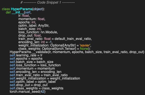
We begin by implementing the HyperParams wrapper class, which encapsulates the hyperparameters used for training and tuning the Graph Convolutional Network. The constructor defines commonly used configuration attributes, including the choice of optimizer, optim_label and, if applicable, the class weight distribution, class_weights to address class imbalance (code snippet 1)
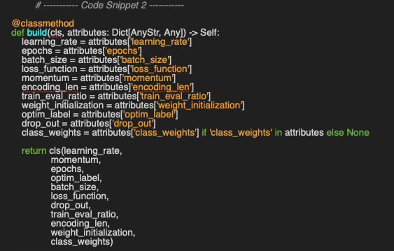
Our plug-and-play approach relies on a detailed configuration for training, implemented through the alternative class method constructor build, which generates a HyperParams instance from a JSON configuration file (code snippet 2).
🔎 Setting up Training
⏭️ This section guides you through the design and code—skip if you only want results.
The GNNTraining class encapsulates the training and validation process, with its default constructor accepting hyper-parameters and metric-related attributes (Code snippet 3). Notably, the alternative build constructor instantiates the training configuration directly from a JSON-formatted string.
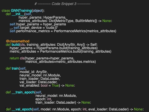
The training and validation process across epochs—controlled by one of the hyper-parameters—is handled by the train method, which accepts the following arguments:
model_id: An identifier for the GNN model, primarily used for debugging
neural_model: The Graph Convolutional Network implemented as a PyTorch module
train_loader: A PyTorch data loader constructed using the train_mask [ref 9]
val_loader: A data loader for validation based on the val_mask.
val_enabled: An optional boolean flag to enable or disable validation
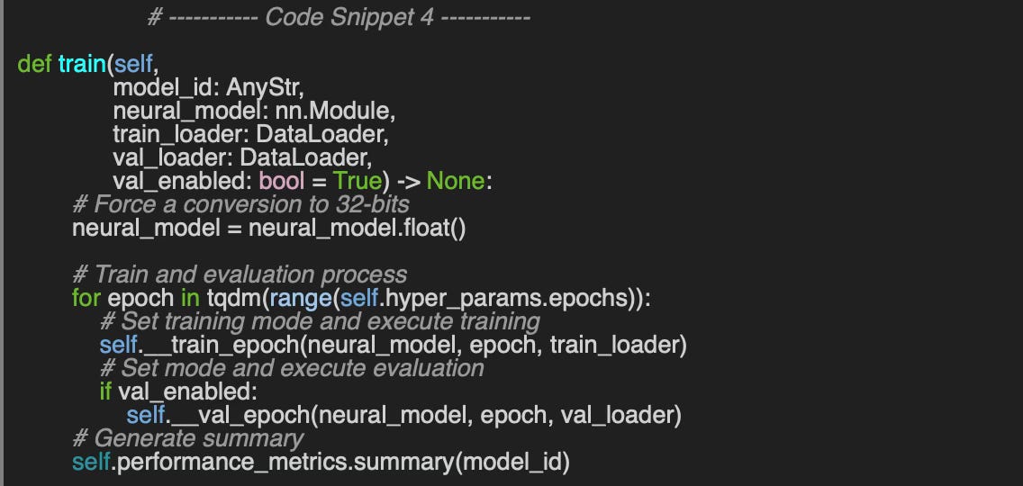
The main loop calls the private method, __train_epoch, which processes batches from the training data loader using the specified hyper-parameters and records the training loss for each epoch.
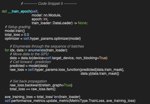
📌 The train_mask has to be applied to both predicted and label data, data.y, Similarly, the val_mask would have to be used on predicted and label validation data.
The implementation of the validation method for each epoch is omitted here. For more details, please refer to the source available at Github.com/patnicolas/dl/training/eval_gconv
Evaluating the Model
The objective is to evaluate a Graph Convolutional Network that can properly classify images from the Flickr Dataset [ref 10]. The Flickr dataset is a graph where nodes represent images and edges signify similarities between them. It includes 89,250 images and 899,756 relationships. Node features consist of image descriptions and shared properties.
🔎 SetUp
We begin by defining the GNNTrainingPlay class to manage model evaluation (Code snippet 6). As expected, its constructor takes two arguments:
_training_attributes: A dictionary containing training settings and hyper-parameter specifications
_sampling_attributes: Defines the data loader and the sampling method.
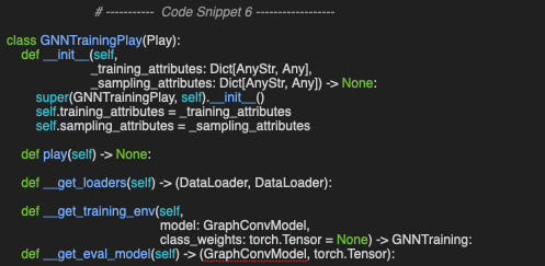
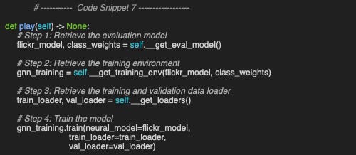
The primary method, play, sequentially calls the following:
__get_loaders: Extracts the training and validation data loaders for the specified dataset (e.g., Flickr)
__get_training_env: Initializes dynamic attributes required for executing training and validation
__get_eval_model: Instantiates the model based on the JSON configuration descriptor.
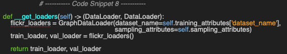
The __get_loaders method leverage the GraphDataLoader class introduced in Demystifying Graph Sampling & Walk Methods: Graph Data Loader
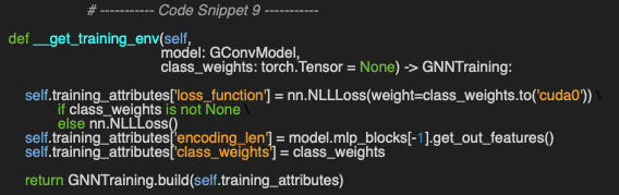
The __get_training_env method defines the remaining three parameters needed to initiate training and set up the environment: the loss function, the number of output classes (encoding_len), and the class weight distribution to address class imbalance.
Our Graph Convolutional Neural Network consists of two graph convolutional blocks followed by a fully connected multilayer perceptron block, as illustrated below.
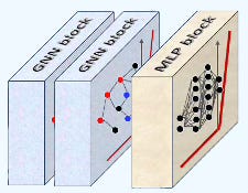
Fig. 2 Illustration of Graph Convolutional Network with two graph convolutional blocks and one fully connected block
The __get_eval_model method loads the dataset using the auxiliary class PyGDatasets [ref 11]. Each of the two graph convolutional blocks includes a hidden layer with 384 units, a ReLU activation function, and dropout regularization set to 0.25—without pooling or batch normalization.
The fully connected block consists of a standard linear layer followed by a LogSoftmax activation module.
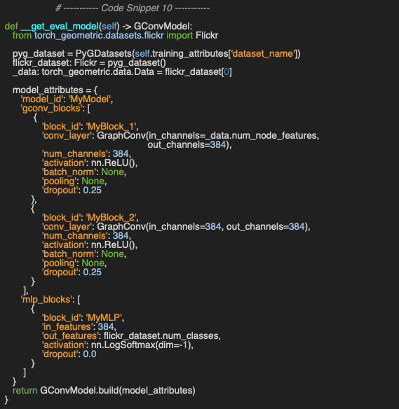
📌 The output layer uses a LogSoftMax activation because the chosen loss function is Negative Log-Likelihood (NLLLoss in PyTorch). In contrast, the standard cross-entropy loss would require a Softmax activation instead.
Results
Finally, training and validation are carried out over 32 epochs using Neighbor Node Sampling, with 12 nodes sampled at the first hop, 6 at the second, and 3 at the third.
 sampling_attributes = {
    'id': 'NeighborLoader',
    'num_neighbors': [12, 6, 3],
    'batch_size': 64,
    'replace': True,
    'num_workers':4
}Accuracy, Precision, Recall, F1 score, along with training and validation losses, are visualized using the widely adopted Matplotlib library.
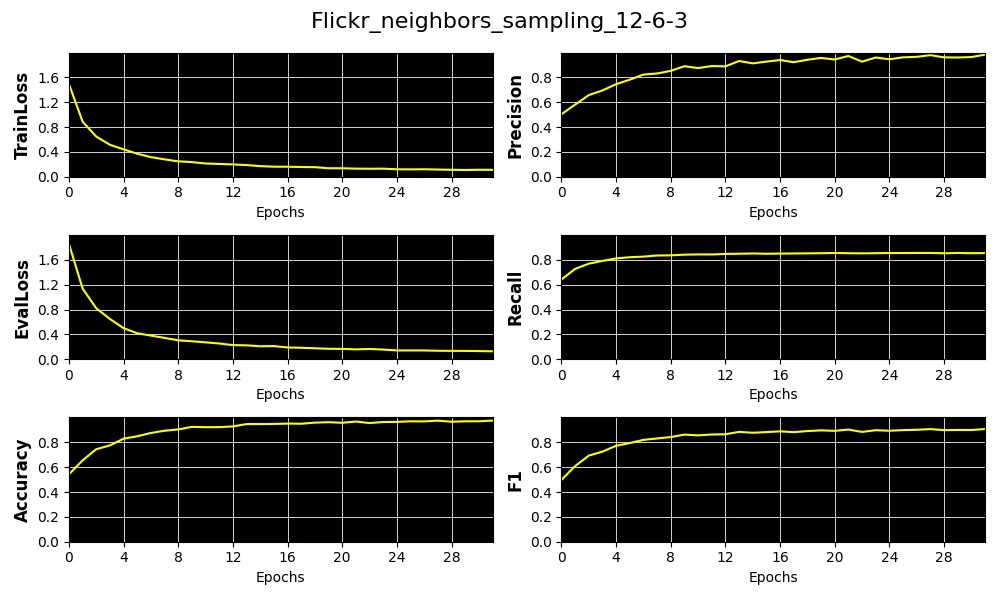
Fig. 3 Output of training and validation of Graph Convolutional Neural Network with Neighbor Node sampling on Flickr data set
🧠 Key Takeaways
✅ Developing a plug-and-play framework for model training and validation accelerates the development cycle and promotes consistency across experiments.
✅ Leveraging a declarative format to specify the training environment, hyper-parameter values, and model structure helps decouple data science tasks from software implementation—minimizing the risk of bugs and reducing the need for redundant testing.
✅ Neural blocks serve as convenient wrappers around PyTorch modules, each corresponding to a specific graph neural network layer.
📘 References
A Practical Tutorial on Graph Neural Networks I. Ward, J. Joyner, C. Lickfold, Y. Guo, M. Bennamoun - 2021
A Comprehensive Introduction to Graph Neural Networks - Datacamp - 2022
Graph Neural Networks: A Gentil Introduction - YouTube. A. Persson
Stanford CS: Machine Learning with Graphs - YouTube - CS-224 Stanford
🛠️ Exercises
Q1: What are the advantages of using a declarative format to define training configurations and model parameters?
Q2: Can you implement class weight computation to balance classes based on their instance counts?
Q3: Which additional hyper-parameters would you consider adding to the attribute list in Code Snippet 2?
Q4: What alternative metric would you recommend for evaluating node classification performance on the Flickr dataset?
Q5: Can you update the JSON model definition in Code Snippet 10 to include a pooling layer of type TopKPooling?
👉 Answers
💬 News & Reviews
This section focuses on news and reviews of papers pertaining to geometric deep learning and its related disciplines.
Paper review: On the Effectiveness of Random Weights in Graph Neural Networks T.Bui, C-B. Schonlieb, B. Ribiero, B. Bevilacqua, M. Elisasof
This paper presents a thought-provoking idea: Can randomly initialized weights in Graph Neural Networks (GNNs) perform as effectively as learned parameters in message-passing layers, while significantly reducing computational training costs?
The proposed approach leverages diagonal weight matrices that preserve key information about message passing, random sampling at each forward pass, and a pretrained node embedding layer.
The model, RAP-GNN (Random Propagation Graph Neural Network), consists of three main components:
Pre-trained embedding layer: Initial node embeddings are generated using a multi-layer perceptron (MLP).
GNN layers stack: A series of message-passing layers interleaved with non-linear activation functions.
Classifier: Operates on node embeddings to make predictions.
Training Process (Two-Stage Approach)
Pre-training: A neural network or single-layer GNN generates node representations.
Training: The classifier is trained while the node representations remain frozen. Instead of computing full weight matrices, a new diagonal matrix of random weights is sampled at each forward pass.
This avoids expensive matrix multiplications and reduces randomness in training.
Key Issues Addressed
Feature Collapse (Homophily): The method increases the rank of the embedding matrix, mitigating homophily effects.
Permutation Equivariance: The approach ensures permutation invariance while still differentiating isomorphic nodes.
Experimental Evaluation
The model is tested on Planetoid, TUDatasets, and OGBN large graphs. The results show that while random sampling of diagonal weights offers only a slight performance improvement, it significantly reduces GPU memory consumption (3x) and training time (6x).
Expertise Level
⭐ Beginner: Getting started - no knowledge of the topic
⭐⭐ Novice: Foundational concepts - basic familiarity with the topic
⭐⭐⭐ Intermediate: Hands-on understanding - Prior exposure, ready to dive into core methods
⭐⭐⭐⭐ Advanced: Applied expertise - Research oriented, theoretical and deep application
⭐⭐⭐⭐⭐ Expert: Research , thought-leader level - formal proofs and cutting-edge methods.
Patrick Nicolas is a software and data engineering veteran with 30 years of experience in architecture, machine learning, and a focus on geometric learning. He writes and consults on Geometric Deep Learning, drawing on prior roles in both hands-on development and technical leadership. He is the author of Scala for Machine Learning (Packt, ISBN 978-1-78712-238-3) and the newsletter Geometric Learning in Python on LinkedIn.