

Graph Convolutional or SAGE Networks? Shootout
Expertise Level ⭐⭐⭐⭐

The right tool for the job! GraphSAGE and Graph Convolutional Network (GCN) are the most commonly used Graph Neural Networks architectures. It is critical to understand the advantages and limitations of each model in order to apply to a specific problem and graph dataset.

🎯 Why this matters
Purpose: Since 2017, countless Graph Neural Network variants have emerged, many implemented in PyTorch Geometric. The challenge is choosing the right model for a given dataset and task. We begin by comparing two staples: GraphSAGE and Graph Convolutional Network (GCN).
Audience: Data scientists and machine learning practitioners exploring or developing Graph Neural Networks.
Value: Learn how to evaluate two graph neural networks across two datasets: a case study of GraphSAGE vs GCN.
🎨 Modeling & Design Principles
Overview
The Graph Convolutional Network (GCN) {ref 1, 2] and GraphSAGE network [ref 3] have been studied in previous articles.
📌 I’ll treat GCN as a representative transductive GNN and GraphSAGE as a canonical inductive model. Comparing other type of GNNs might have produced different results.
Inductive vs. Transductive
Inductive graph neural networks learn from existing (training) and new, unseen nodes, links or graphs (inference) [ref 4]. There is no need for these models to store and node/link embeddings. The graph SAGE model that leverages PyTorch Geometric is strictly inductive.
Transductive graph models are trained on the complete, fully defined graph (all nodes and edges). As a result, they tend to overfit the training set and struggle to generalize to unseen nodes, edges, or entirely new graphs. Their message passing and aggregation schemes are typically straightforward. Our PyTorch Geometric implementation of the Graph Convolutional Network follows this transductive setting.
A brief comparison between GCN and GraphSAGE was presented in a previous article [ref 5]. Here is a different perspective:
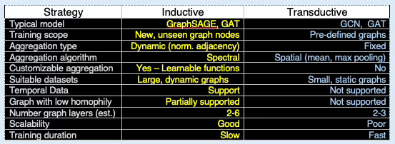
Table 1 Comparison attributes of inductive (GraphSAGE) and transductive (GCN) models
📌 Some of graph neural network (e.g., GAT) can run inductively and transductively, although they tend to be evaluated as transductive graphs.
Evaluation Configuration
The objective is to compare the performance of GCN and GraphSAGE models for classifying nodes, given a set of dynamic evaluation parameters.
Model Parameters for Evaluation
Using the strengths of GraphSAGE and GCN outlined above, we set our evaluation knobs as follows.
Homophily: GraphSAGE is more robust on low-homophily graphs thanks to learnable aggregators (e.g., mean, sum), whereas GCN tends to degrade.
Network Depth: GraphSAGE often benefits from deeper stacks of graph layers than its convolutional counterpart.
Neighborhood scope: The depth vs. fan-out of sampling materially affects node-classification performance.
Size of the graph: GCN leverages the entire graph during training and therefore consumes significantly more memory.
📌 The choice of message aggregator (e.g., mean, GCN-style, max-pool) affects the performance of inductive models like GraphSAGE. We encourage readers to experiment with different aggregation functions.
Performance Metrics
We are using the following performance metrics: Accuracy, Precision, Recall, F1, Area under the ROC curve and Area under Precision/Recall curve.
📌 We make no task-specific assumptions (node classification, link prediction, etc.); instead, we use the most common performance metrics to ensure a consistent comparison.
Datasets
We select two well-known datasets from PyTorch Geometric library
Cora, a small graph with high homophily. This is a standard benchmark dataset for semi-supervised node classification, containing 2,708 nodes (scientific publications) and 5,429 edges (citations). Each node is described by a 1,433-dimensional feature vector. GCN’s full-batch, Laplacian-based propagation matches this regime and typically edges out or matches GraphSAGE while being simpler. This dataset is also included in torch_geometric.datasets.Planetoid class collection.
Flickr, a large graph with low homophily. This dataset contains descriptions and common properties of 89,250 images along with 899.756 edges and a 500-dimensional feature vector. It is defined in torch_geometric.datasets.Flickr class. GraphSAGE commonly trained with mini-batch neighbor sampling of Flickr.
Homophily is not as high as citation graphs, so simple Laplacian smoothing (GCN) can be less effective; SAGE’s learnable aggregations (mean/max/attention or “gcn” variant) tend to be more robust.
Cora node homophily: 0.825
Cora edge homophily: 0.810
Cora edge_insensitive homophily: 0.766

Flickr node homophily: 0.322
Flickr edge homophily: 0.319
Flickr edge_insensitive homophily: 0.070
⚙️ Hands‑on with Python
Environment
Libraries: Python 3.12.5, PyTorch 2.5.0, Numpy 2.2.0, Networkx 3.4.2, PyTorch Geometric 2.5.0
Source code: geometriclearning/deeplearning/model/graph/graph_sage_model.py
geometriclearning/deeplearning/model/graph/graph_conv_model.py
Evaluation code: geometriclearning/play/graph_sage_vs_gcn_play.py
The source tree is organized as follows: features in python/, unit tests in tests/, and newsletter evaluation code in play/.
To enhance the readability of the algorithm implementations, we have omitted non-essential code elements like error checking, comments, exceptions, validation of class and method arguments, scoping qualifiers, and import statements.
🔎 Architectural Design
⏭️ This section guides you through the design and code.
Reusable neural blocks and model builders are essential for creating modular, configurable graph neural networks. Let’s take a closer look at these concepts.
Graph Neural Blocks
Reusable neural blocks, introduced in [ref 6], provide a simple and convenient way to package related PyTorch components into modular units that can be dynamically assembled for efficient model development.
In our framework, a graph neural block typically includes a message passing and aggregation module, along with optional PyTorch layers such as activation, batch normalization, and dropout.
From a software design perspective, both GraphSAGEBlock [ref 7] (for GraphSAGE) and GraphConvBlock (for GCN) inherit from a common base class, MessagePassingBlock.
This base class organizes four core components:
message_passing_module: the message passing operator (e.g., GraphConv, GCNConv for GCN; SAGEConv, CuGraphSAGEConv for GraphSAGE)
batch_norm_module: optional batch normalization
activation_module: optional activation function (e.g., ReLU, LeakyReLU)
dropout_module: optional node-level dropout regularization.
The following class diagram, Figure 1, illustrates the relation between the various block and torch modules
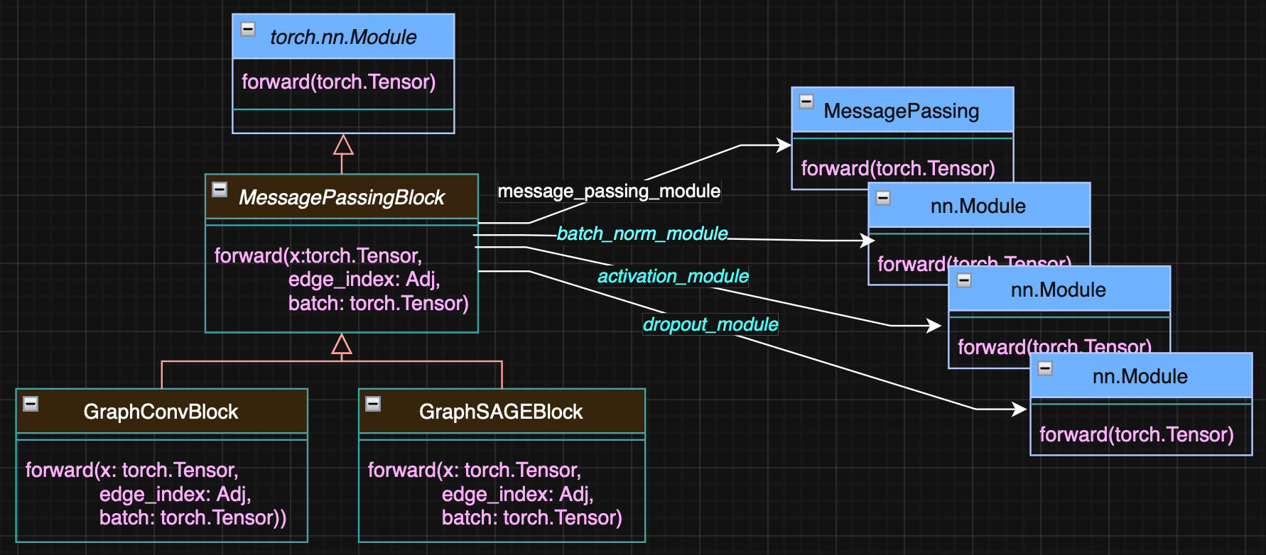
Fig. 1 Class diagram for Graph Convolutional and SAGE neural blocks
The optional attributes of the base class MessagePassingBlocks — Activation, Batch Normalization, and Dropout — are shown in italic and highlighted in cyan.
Contrary to traditional neural model such as convolutional network or multilayer perceptron, the forward method has to accommodate a graph structure. The arguments are
x: Stacked node feature vectors for the entire graph
edge_index: Adjacency matrix describing all edges
batch: A PyTorch geometric specific feature to keep track which node belong to which graphs
Graph Neural Models
All graph neural network model classes inherit from the abstract base class GraphBaseModel. They share a common training and validation method, train_model, which relies on the utility class GNNTraining introduced in a previous article [ref 8].
The forward method can be overridden in specific models. It iteratively applies message-passing blocks (derived from MessagePassingBlock) along with fully connected layers implemented as instances of MLPBlock.
The relationship between the various class-models and their component is illustrated in Figure 2.
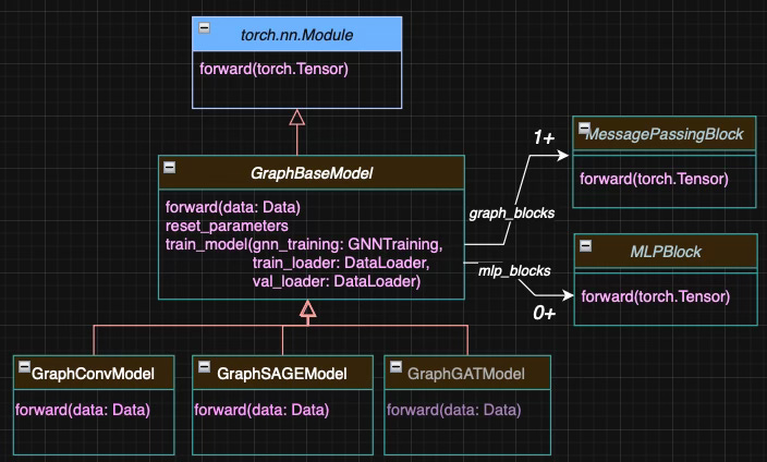
Fig. 2 Class diagram for Graph Convolutional and SAGE models
As with article focuses on comparing two Graph Neural Networks, hyper-parameters optimization is out of scope [ref 9]. Therefore, we fix the training hyper-parameters to commonly recommended values. A detailed article on hyper-parameter optimization using Optuna is available in this newsletter: How to Tune a Graph Convolutional Network
training_attributes = {
    'dataset_name': dataset_name,
            # Model training Hyperparameters
    'learning_rate': 0.001,
    'batch_size': 64,
    'loss_function': nn.CrossEntropyLoss(label_smoothing=0.05,
                                         reduction='mean'),
    'momentum': 0.95,
    'weight_decay': 5e-4,
    'train_eval_ratio': 0.9,
    'weight_initialization': 'kaiming',
    'optim_label': 'adam',
    'drop_out': 0.4,
    'is_class_imbalance': True,
    'class_weights': class_weights,
    'epochs': 40,
            # Model configuration
    'hidden_channels': 256,
            # Performance metric definition
    'metrics_list': [
        'Accuracy', 'Precision', 'Recall', 'F1', 'AuROC', 'AuPR'
     ]
}
The implementation of the evaluation leverages the neural blocks (GraphConvBlock and GraphSAGEBlock) introduced in previous articles [ref 7].
🔎 Test Code
👉 The evaluation code available at geometriclearning/play/graph_sage_vs_gcn_play.py
Here are some excerpts to help reader navigate GitHub repository.
Setup
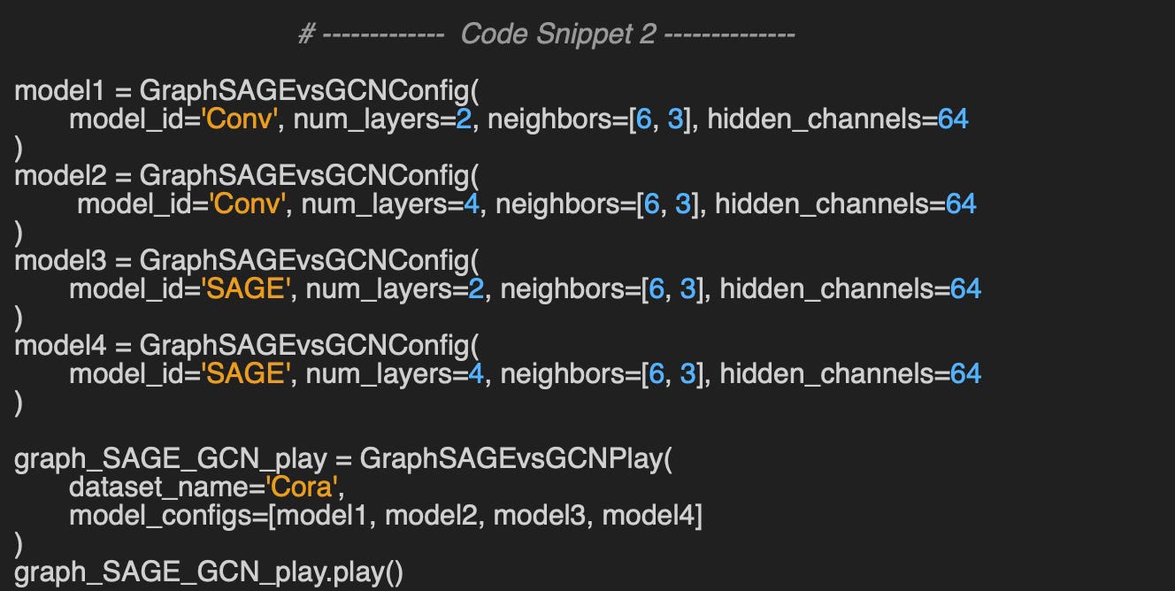
We wrap the parameters used in the evaluation of the two graph neural networks into a data class GraphSAGEvsGCNConfig.
model_id: Identifier for the model
num_layers: Depth (number of graph neural layers) of the model
neighbors: List of neighboring nodes and fanout for message aggregation
hidden_channels: Number of channels or neurons in graph and fully connected layers.
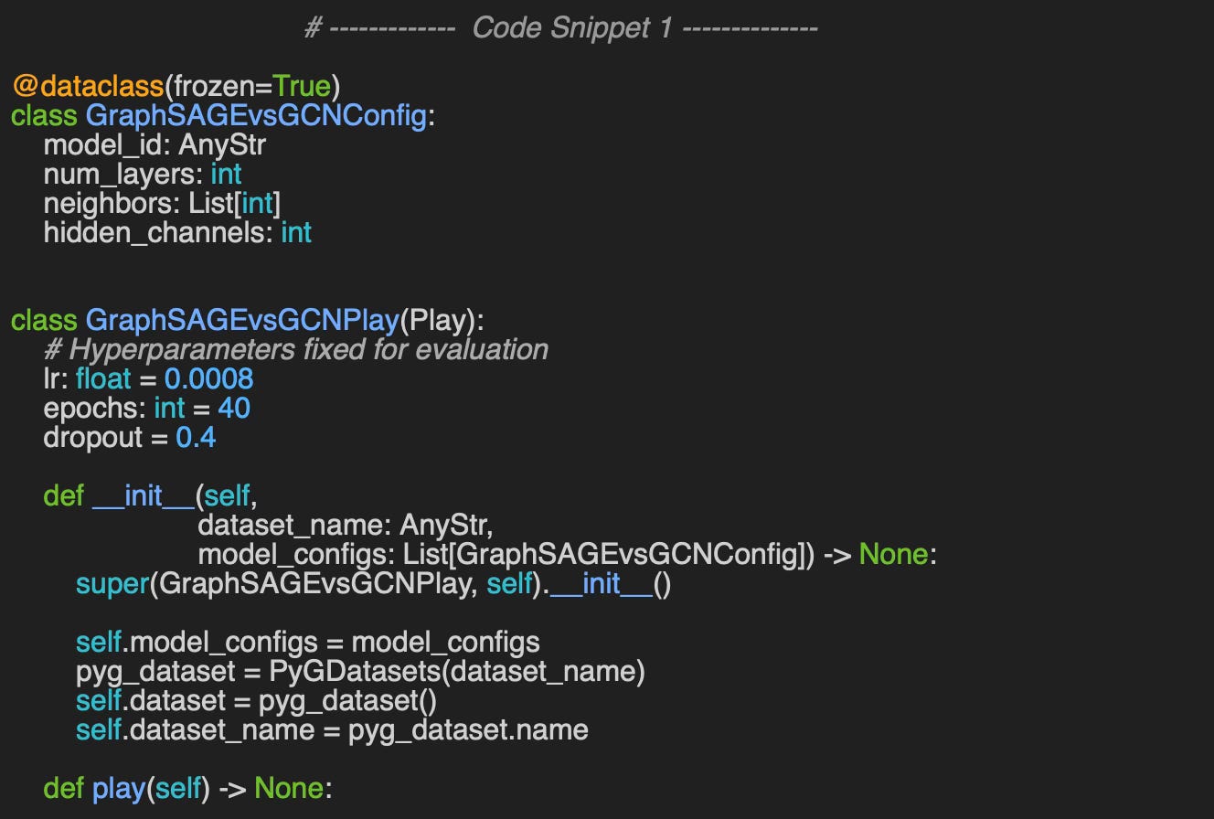
The class GraphSAGEvsGCNPlay encapsulates the relative evaluation of GraphSAGE and GCN models. The constructor has 2 arguments
dataset_name: Name of the PyTorch Geometric graph data used for evaluation (Cora or Flickr)
model_configs: List of model configurations.
Here is example of Graph neural network configuration used in the evaluation.
The method play does the heavy lifting: Load the training parameters, followed by the model parameters and neighborhood sampling parameters, specified as JSON string (Dictionary) [ref: geometriclearning/play/graph_sage_vs_gcn_play.py ]
GraphSAGE configuration
As a reminder, a neural block for a GraphSAGE - instance of GraphSAGEBlock - is composed of
block_id: Identifier
SAGE_layer: PyTorch Geometric SAGE convolutional module
batch_norm: Optional Batch normalization module
activation: PyTorch activation module/function
dropout: Optional PyTorch dropout regularization module.
The output blocks, mlp_blocks consists of a single PyTorch linear module, layer_module without an activation function.
{
   'model_id': 'GraphSAGE',
   'graph_SAGE_blocks': [
      {
        'block_id': 'SAGE Layer 1',
        'SAGE_layer':SAGEConv(in_channels=dataset[0].num_node_features,
                              out_channels=hidden_channels),
        'num_channels': hidden_channels,
        'activation': nn.ReLU(),
        'batch_norm': None,
        'dropout': 0.4
      },
      {
        'block_id': 'SAGE Layer 2',
        'SAGE_layer': SAGEConv(in_channels=hidden_channels,
                              out_channels=hidden_channels),
        'num_channels': hidden_channels,
        'activation': nn.ReLU(),
        'batch_norm': None,
        'dropout': 0.4
      }
   ],
   'mlp_blocks': [
      {
        'block_id': 'Node classification block',
        'in_features': hidden_channels,
        'out_features': dataset.num_classes,
        'activation': None
      }
   ]
}
GCN configuration
Similarly, GraphSAGE block, instance of GraphConvBlock is composed of
block_id: Identifier
conv_layer: PyTorch Geometric graph convolutional module
batch_norm: Optional Batch normalization module
activation: PyTorch activation module
pooling: Optional pooling module
dropout: Optional PyTorch dropout regularization module.
{
  'model_id': 'GCN',
  'graph_conv_blocks': [
     {
       'block_id': 'MyBlock_1',
       'conv_layer': GraphConv(in_channels=_data.num_node_features,
                               out_channels=hidden_channels),
       'num_channels': hidden_channels,
       'activation': nn.ReLU(),
       'batch_norm': None,
       'pooling': None,
       'dropout': 0.4
     },
     {
       'block_id': 'MyBlock_2',
       'conv_layer': GraphConv(in_channels=hidden_channels,
                               out_channels=hidden_channels),
        'num_channels': hidden_channels,
        'activation': nn.ReLU(),
        'batch_norm': None,
        'pooling': None,
        'dropout': 0.4
      }
    ],
    'mlp_blocks': [
      {
         'block_id': 'Output',
         'in_features': hidden_channels,
         'out_features': dataset.num_classes,
         'activation': None
      }
   ]
}
📈 Evaluation
For this evaluation the GCN and GraphSAGE uses ReLU activation and a dropout regularization factor 0.4. No pooling layer is used for the GCN [ref 11].
⚠️ We do not tune common hyperparameters (e.g., learning rate, early-stopping) in this evaluation; fine-tuning isn’t necessary for isolating which factors drive the relative performance of GraphSAGE vs. GCN.
Cora Dataset
Configuration 1:
Small graph with small neighborhood sampling and 2/4 graph neural layers
GraphSAGE: Neighborhood hop/fanout [6, 3], 2 Graph Neural Layers
GraphSAGE: Neighborhood hop/fanout [6, 3], 2 Graph Neural Layers
GCN: Neighborhood hop/fanout [6, 3], 2 Graph Neural Layers
GCN: Neighborhood hop/fanout [6, 3], 4 Graph Neural Layers
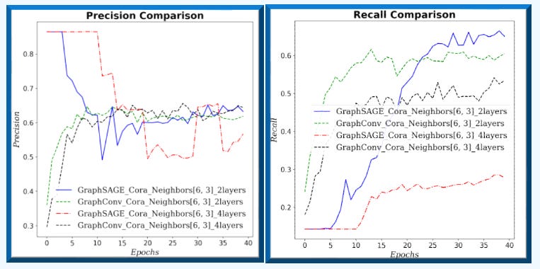
Fig. 3 Precision-Recall for GraphSAGE and GCN for neighborhood sampling (6, 3) and 2/4 graph layers for Cora dataset.

Fig. 4 Accuracy & F1 measure for GraphSAGE and GCN for neighborhood sampling (6, 3) and 2/4 graph layers for Cora dataset.
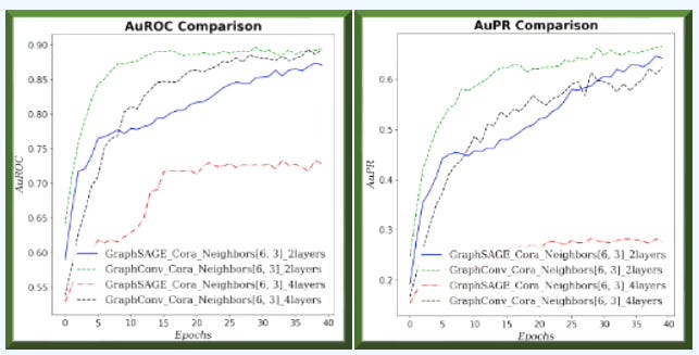
Fig. 5 Area under ROC and Precision/Recall curves for GraphSAGE and GCN for neighborhood sampling (6, 3) and 2/4 graph layers for Cora dataset.
Configuration 2:
Small graph with larger neighborhood sampling and 2/4 graph neural layers
GraphSAGE Neighborhood hop/fanout [20, 12], 2 Graph Neural Layers
GraphSAGE Neighborhood hop/fanout [20, 12], 4 Graph Neural Layers
GCN Neighborhood hop/fanout [20, 12], 2 Graph Neural Layers
GCN Neighborhood hop/fanout [20, 12], 4 Graph Neural Layers
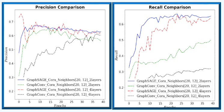
Fig. 6 Precision-Recall for GraphSAGE and GCN for neighborhood sampling (20, 12) and 2 graph layers for Cora dataset.
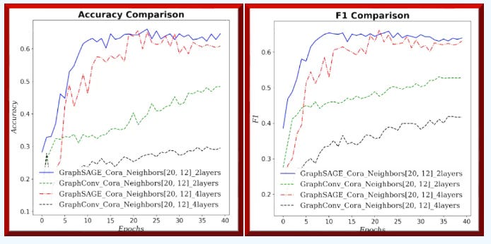
Fig. 7 Accuracy & F1 measure for GraphSAGE and GCN for neighborhood sampling (20, 12) and 2 graph layers for Cora dataset.
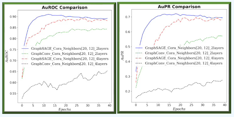
Fig. 8 Area under ROC and PR curves for GraphSAGE and GCN for neighborhood sampling (20, 12) and 2 graph layers for Cora dataset.
Outcome
On small graphs with limited neighborhoods (few neighbors, low fanout), GCN has the edge. As the receptive field grows—more hops and higher fanout—GraphSAGE improves relative to GCN.
📌 We train each model for 40 epochs to compare behavior rather than fine-tune; longer runs don’t materially change the results.
Flickr Dataset
Configuration 3:
Larger graph with small neighborhood sampling and 2/4 graph neural layers
GraphSAGE Neighborhood hop/fanout [12, 6], 2 Graph Neural Layers
GraphSAGE Neighborhood hop/fanout [12, 6], 2 Graph Neural Layers
GCN Neighborhood hop/fanout [12, 6], 2 Graph Neural Layers
GCN Neighborhood hop/fanout [12, 6], 4 Graph Neural Layers
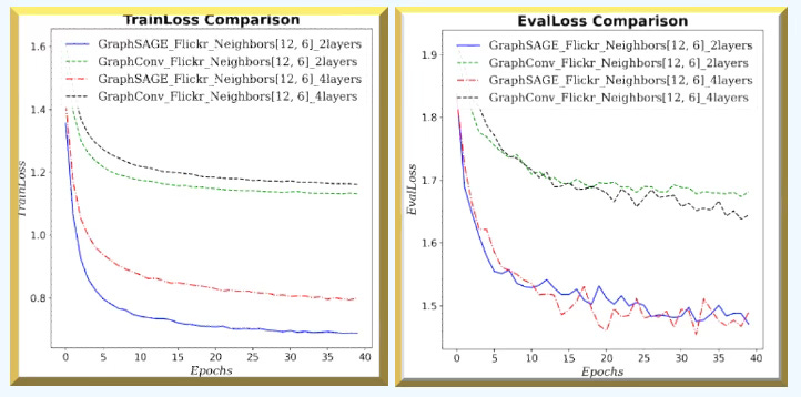
Fig. 9 Training & validation losses for GraphSAGE and GCN with (12, 6) neighbors sampling and 2 or 4 graph neural layers for Flickr dataset - Node classification
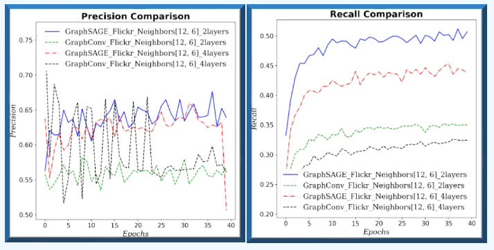
Fig. 10 Precision & Recall for GraphSAGE and GCN with (12, 6) neighbors sampling and 2 or 4 graph neural layers for Flickr dataset - Node classification
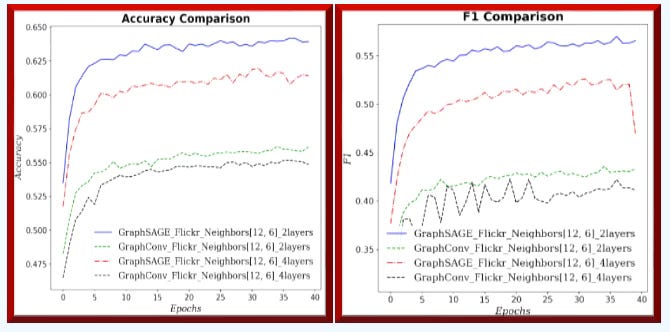
Fig. 11 Accuracy and F1 metric for GraphSAGE and GCN with (12, 6) neighbors sampling and 2 or 4 graph neural layers for Flickr dataset - Node classification
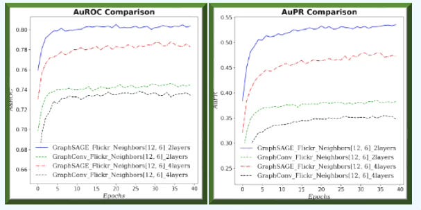
Fig. 12 Area under ROC and Precision/Recall curves for GraphSAGE and GCN with (12, 6) neighbors sampling and 2 or 4 graph neural layers for Flickr dataset - Node classification
Outcome
GraphSAGE consistently and significantly outperforms GCN across all metrics and loss values for large graph (Flickr). In addition, increasing the number of GNN layers/blocks degrades performance.
🧠 Key Takeaways
✅ On small graphs with a limited neighborhood scope, GCN tends to perform better; however, GraphSAGE improves as you increase the number of neighbors per hop and the fanout
✅ GraphSAGE clearly outperforms GCN on large graphs.
✅ In our tests on two PyTorch Geometric datasets, adding more layers to either GCN or GraphSAGE did not yield gains.
✅ PyG’s GitHub includes a section comparing methods under homogeneous evaluation (see [ref 12]).
✅ Our experiments used a single sampling strategy—torch_geometric.loader.NeighborLoader—but readers are encouraged to try alternative loaders/samplers.
📘 References
A Gentle Introduction to Graph Neural Networks B. Sanchez-Lengeling, E. Reif, A. Pearce, A. Wiltschko - Distill - 2021
An introduction to Robust Graph Convolutional Networks M. Najafi, P. S. Yu - University of Illinois at Chicago - 2021
Revisiting Inductive Graph Neural Networks Hands-on Geometric Deep learning - 2025
Inductive Representation Learning on Large Graphs W. Hamilton, R. Ying, J. Leskovec - Dept. of Computer Science - Stanford University - 2017
Graph SAGE vs Graph Convolution Hands-on Geometric Deep learning - 2025
Graph Neural Network Neural Components Hands-on Geometric Deep learning - 2025
GraphSAGE block Hands-on Geometric Deep learning - 2025
Plug & Play Training for Graph Convolutional Networks Hands-on Geometric Deep learning - 2025
How to Tune a Graph Convolutional Network Hands-on Geometric Deep learning - 2025
GraphSAGE Model Hands-on Geometric Deep learning - 2025
Taming Graph Neural Networks with PyTorch Geometric - Graph Datasets Hands-on Geometric Deep learning - 2025
🛠️ Q&A
Q1: What are the key differences between transductive and inductive graphs?
Q2: For low-homophily graphs, which GNN is more suitable—GCN or GraphSAGE?
Q3: Do hyperparameters like learning rate or number of epochs affect the relative comparison between two GNNs?
Q4: Which evaluation metrics are best for comparing two models?
Q5: On large graphs, does GCN outperform GraphSAGE?
Q6: How does increasing the number of neighbors and fanout for message aggregation influence the comparison between GraphSAGE and GCN?
💬 News & Reviews
This section focuses on news and reviews of papers pertaining to geometric deep learning and its related disciplines.
Paper Review: Feature-Based Lie Group Transformer for Real-World Applications T. Komatsu, Y. Ohmura, K. Nishitsunoi, Y. Kuniyoshi - Graduate School of Information Science and Technology, University of Tokyo - 2025
The authors introduce a straightforward method that integrates feature extraction and object segmentation to replace traditional pixel-wise transformations in image classification.
This approach—termed feature-based transformation—is applied to a sequence of scene images as follows:
An object is segmented from the first scene image using a binary mask.
The object is divided into an N×N grid of patches.
Each patch is encoded into a feature vector.
The feature representation of the first image is used to transform the features of subsequent images.
These transformed features yield the updated object representation and mask.
Their method is grounded in the concepts of conditional independence and Lie group transformations (specifically translation and rotation), implemented via Neural Ordinary Differential Equations (Neural ODEs).
The evaluation is conducted under constrained conditions:
Pixel-to-pixel transformations
A single object per image
Low resolution with minimal background
Test cases include:
A synthetic object without background
A real-world object with background
Reader classification rating
⭐ Beginner: Getting started - no knowledge of the topic
⭐⭐ Novice: Foundational concepts - basic familiarity with the topic
⭐⭐⭐ Intermediate: Hands-on understanding - Prior exposure, ready to dive into core methods
⭐⭐⭐⭐ Advanced: Applied expertise - Research oriented, theoretical and deep application
⭐⭐⭐⭐⭐ Expert: Research , thought-leader level - formal proofs and cutting-edge methods.
Share the next topic you’d like me to tackle.
Patrick Nicolas is a software and data engineering veteran with 30 years of experience in architecture, machine learning, and a focus on geometric learning. He writes and consults on Geometric Deep Learning, drawing on prior roles in both hands-on development and technical leadership. He is the author of Scala for Machine Learning (Packt, ISBN 978-1-78712-238-3) and the newsletter Geometric Learning in Python on LinkedIn.