

How to Tune a Graph Convolutional Network

Does tuning the hyperparameters for a Graph Convolutional Neural Network feel like searching for a needle in a haystack?
This article guides you through different hyperparameter optimization (HPO) techniques and shows how to break down the search space into manageable parts


🎨 Modeling & Design Principles
Graph Convolutional Neural Networks
🛠️ Exercises

🎯 Why this Matters
Purpose: Simplify the complexity of hyperparameter optimization (HPO) for Graph Convolutional Networks with a structured approach and a lightweight yet powerful Python library.
Audience: Data scientists and engineers facing the daunting task to optimize the various parameters of a Graph Convolutional Network
Value: Learn how to explore the most widely used HPO algorithms, decompose the search space into manageable components, and apply Optuna to fine-tune a key parameter in GCNs: neighbor node sampling.
🎨 Modeling & Design Principles
⚠️ I strongly recommend to review my articles introducing PyTorch Geometric Taming PyTorch Geometric for Graph Neural Networks and Graph loaders Demystifying Graph Sampling & Walk Methods
Overview
Tuning hyperparameters for a Graph Convolutional Neural Network can feel like searching for a needle in a haystack—overwhelming and complex. To navigate this challenge effectively, it's essential to understand the model’s behavior, identify which parameters truly impact performance, and choose a suitable optimization strategy.
Graph Convolutional Neural Networks
Graph Neural Networks have been discussed in depth in previous articles in this newsletter [ref 1, 2]
A Graph Neural Network (GNN) is an optimizable transformation on all attributes of the graph (nodes, edges, global context) that preserves graph symmetries (permutation invariances). GNN takes a graph as input and generate/predict a graph as output.
Data on manifolds can often be represented as a graph, where the manifold's local structure is approximated by connections between nearby points. GNNs and their variants (like Graph Convolutional Networks (GCNs) extend neural networks to process data on non-Euclidean domains by leveraging the graph structure, which may approximate the underlying manifold.
The generation of universal embeddings that apply across different applications remains a significant challenge.
PyTorch Geometric simplifies this process by encapsulating these complexities into specialized data loaders, while seamlessly integrating with PyTorch's existing deep learning modules.
👉 This study uses a Graph Convolutional Network applied on Flickr dataset
Hyperparameter Optimization (HPO)
Overview
Hyperparameter optimization (HPO) is the automated process of identifying the most effective configuration settings—like learning rate, batch size, or number of layers—for training a machine learning model. Think of it as fine-tuning the dials on your model to ensure it learns optimally and delivers the best performance.
Hyperparameters are key configuration variables that control the learning behavior of machine learning algorithms. Manually searching for good hyperparameter values is often inefficient and quickly becomes impractical as the number of options grows. Automating this search is essential to make machine learning more scalable, reproducible, and less reliant on trial-and-error. It also empowers researchers and practitioners to focus on higher-level tasks instead of low-level tuning [ref 4].
Hyperparameters have a profound impact on model performance—not only in terms of generalization, but in determining what may qualify as state-of-the-art.
However, hyperparameter optimization comes with significant challenges:
The objective function often lacks a tractable analytical form.
It may contain multiple local optima.
The search landscape can include flat regions or saddle points.
The objective function may be non-smooth or even discontinuous.
Efficiency and Multi-fidelity
Hyperparameter optimization (HPO) can be computationally expensive, especially when dealing with large datasets, numerous hyperparameters, or complex model architectures. To manage resource consumption, development teams often set a fixed budget for HPO to prevent exhausting available compute capacity.
One effective strategy to reduce the cost of HPO is to approximate the objective function. For example, many hyperparameter configurations can be evaluated using a limited number of training epochs. As promising candidates emerge, the number of epochs is gradually increased for a more refined evaluation. This cost-saving approach is known as multi-fidelity optimization.
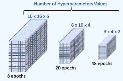
Fig. 1 Illustration of multi-fidelity hyperparameter optimization
Grid Search
Grid search involves evaluating the objective function across a predefined set of hyperparameter configurations. The search space is formed by taking the Cartesian product of all specified values for each hyperparameter, resulting in a grid of possible combinations. The learning algorithm is then applied to each configuration, either sequentially or in parallel, to identify the most effective set of parameters.
Random Search
Random search works by repeatedly sampling hyperparameter configurations from predefined probability distributions. Since the search is stochastic and could, in principle, continue indefinitely, it's typically constrained by a termination condition—such as a time limit or a maximum number of trials. Compared to grid search, random search is generally more efficient in high-dimensional spaces where the number of hyperparameters is large.
Quasi-Random Search
Quasi-random search methods aim to blend the strengths of both grid and random search by using sampling strategies that mix randomness with deterministic structure. These methods generate quasi-random sequences—designed to cover the search space more uniformly than purely random samples. In hyperparameter optimization, they have been shown to consistently outperform standard random search (based on uniform distributions) across various deep learning tasks.
Sobol Sequences
Sobol sequences are a type of low-discrepancy, quasi-random sequence used to sample points in a multi-dimensional space more uniformly than purely random sampling. In hyperparameter optimization, they provide a systematic and efficient way to explore the search space.
Instead of drawing points randomly (which can leave gaps or clusters), Sobol sequences aim to evenly fill the space, ensuring better coverage with fewer evaluations.
Bayesian Optimization
Bayesian Optimization is a probabilistic, model-based strategy for efficiently searching the hyperparameter space. It is especially useful when evaluating each set of hyperparameters is expensive (e.g., deep learning training).
Rather than randomly sampling or exhaustively testing combinations, Bayesian optimization builds a surrogate model(typically a probabilistic model like a Gaussian Process or Tree-structured Parzen Estimator) to estimate the performance of hyperparameter configurations.
'
The process is as follow:
Initialize hyperparameter configurations with a small number of random trails
Create a surrogate model of the objective (or loss) function based on past evaluations
Apply an acquisition function such as Upper Confidence Bound to select the next hyperparameter configuration, balancing exploration and exploitation
Evaluate the selected configuration using the original objective function
Update the surrogate model with new batch of data.
📌 Two types of surrogate models are commonly used in Bayesian Optimization.
Traditional Gaussian Process (GP)
Tree-Structured Parzen Estimator (TPE), a non-parametric, density-based model
Evolutionary Algorithms
This class of algorithms can be broken down into two groups:
Evolutionary Strategies (ES)
Genetic Algorithms (GA)
Genetic Algorithms (GA) are a class of optimization methods primarily designed for binary or discrete search spaces, whereas Evolution Strategies (ES) focus on real-valued, continuous objective functions.
Common transformation types in evolutionary algorithms, which together support the balance between exploration and exploitation, include:
Selection: A global operation that filters out individuals with low fitness and selects the more promising ones to serve as "parents" for the next generation.
Recombination (or crossover): A global transformation that creates new individuals by combining parts—such as subsets of hyperparameter values—from two or more parent solutions.
Mutation: A local modification technique that introduces random changes (e.g., adding Gaussian noise) to individuals. This helps avoid getting trapped in local optima and encourages exploration.
Additional strategies, such as elitism, may also be employed to preserve the best individuals across generations.
📌 The terminology used in evolutionary algorithms (EA) is inspired by biology: a group of candidate solutions is referred to as a population, and each individual configuration is called an individual, chromosome, or genotype. Each iteration of the algorithm is known as a generation, and the objective function is termed the fitness function.
Static & Dynamic Hyperparameters Initialization
Optimizing the many parameters involved in training and evaluating a Graph Neural Network can be daunting—even for experienced practitioners. To simplify this process, we divide the search for the optimal architecture and training configuration into three distinct steps, as outlined below:
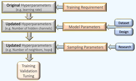
Fig. 2 Three step optimization process for architecture design, training and configuration of a Graph Neural Network.
Most parameters—such as the learning rate—are independent of the sampling strategy or dataset and can be defined statically. However, some training parameters, like the loss function or class weights, are determined dynamically after the data is loaded and analyzed. Likewise, data scientists may impose constraints on hyperparameter optimization (HPO) by predefining the architecture of neural layers or incorporating insights from prior research.
⚙️ Hands-on with Python
Environment
Libraries: Python 3.11.8, PyTorch 2.1.0, PyTorch Geometric 2.6.1, Optuna 4.2.0
Source code: geometriclearning/deeplearning/training/gnn_tuning.py
Evaluation code: geometriclearning/play/gnn_tuning_play.py
The source tree is organized as follows: features in python/, unit tests in tests/,and newsletter evaluation code in play/.
To enhance the readability of the algorithm implementations, we have omitted non-essential code elements like error checking, comments, exceptions, validation of class and method arguments, scoping qualifiers, and import statements.
⚠️ Warning: Some sampling methods in PyTorch Geometric rely on additional modules: torch-sparse, torch-scatter, torch-spline-conv, and torch-cluster. These are dependencies of torch-geometric but they may not be compatible with the latest versions of PyTorch, particularly across different operating systems.
For macOS, we recommend the following version setup for best compatibility:
Python: 3.11.8
PyTorch: 2.1.0
torch-geometric: 2.6.1
torch-sparse: 0.6.18
torch-scatter: 2.1.2
torch-spline-conv: 1.2.2
torch-cluster: 1.6.3
These modules currently support only CPU and CUDA execution — MPS (Metal) is not supported.
Optuna Library
We chose Optuna —an open-source framework—for automating hyperparameter optimization due to its simplicity and broad support for various algorithms, including [ref 5]:
Grid search
Random search
Tree-structured Parzen Estimator (TPE) without constraints
Gaussian process-based Bayesian optimization with inequality constraints
Random forest-based Bayesian optimization
The tutorial also features a comprehensive and engaging example of Human-in-the-Loop Optimization using interactive widgets [ref 6].
To install: pip install optuna
The framework has a dashboard, Optuna-Dashboard to monitor
To install: pip install optuna-fast-fanova gunicorn
📌 The most common alternative hyper parameter optimization libraries are
Ray Tune A scalable engine supporting Grid, Random and Bayesian optimization, designed for large scale multi-node experiments.
Hyperopt A Distributed Asynchronous Hyper-parameter Optimization engine that leverages Apache Spark and MongoDB to distributed optimization runs. It supports the Tree of Parzen Estimators (TPE), Adaptive TPE and Random Search
Nevergrad An optimization solution based on evolutionary and genetic algorithms (Gradient free) with support for mixed continuous and categorical parameters.
SciKit-learn Optimize An module of Scikit learn library that supports Random, Grid and Halving search
Hyperparameters Categories
The different types of parameters involved in configuring, training, and validating a model are thoroughly discussed in a previous article [ref 7]. For clarity, we categorize these parameters into three main groups:
Training parameters — such as the learning rate, which govern the optimization process.
Model parameters — such as the number of graph convolutional layers, which define the architecture.
Sampling methods (Graph Neural Model)— such as Graph Sampling-Based Inductive Learning, which influence how data is fed into the model.
📌 We separate model parameters from sampling methods, both of which are intrinsic to graph-based models, in order to decompose the search space into more manageable components.
Training parameters
Training parameters refer to the configuration settings that control the execution of training and validation processes, including aspects like the learning rate, number of epochs, and convergence criteria. Here is an example:
{
  'dataset_name': 'Sonar',
  'learning_rate': 0.0005,
  'batch_size': 64,
  'loss_function': nn.NLLLoss(weight=class_weights.to('cuda0')),
  'momentum': 0.90,
  'encoding_len': 8,
  'train_eval_ratio': 0.9,
  'weight_initialization': 'xavier',
  'optim_label': 'adam',
  'drop_out': 0.25,
  'is_class_imbalance': True,
  'class_weights': [0.25, 0.3, 0.2, 0.2, 0.05],
  'metrics_list': ['Accuracy', 'Precision', 'Recall', 'F1'],
   ....
}
Model Parameters
In this newsletter, deep learning models are structured as a sequence of neural blocks, and Graph Neural Networks follow the same modular design [ref 8, 9].
The JSON example below outlines a series of graph convolutional and fully connected (multi-layer perceptron) blocks, each linked to specific PyTorch modules such as linear or convolutional layers, activation functions, pooling, or dropout
{
   'model_id': 'my_model',
   'gconv_blocks': [
      {
        'block_id': 'MyBlock_1',
        'conv_layer': GraphConv(in_channels=num_node_features,
                                out_channels=hidden_channels),
        'num_channels': hidden_channels,
        'activation': nn.ReLU(),
        'batch_norm': None,
        'pooling': None,
        'dropout': 0.25
      },
      .....
   ],
   'mlp_blocks': [
      {
        'block_id': 'MyMLP',
        'in_features': hidden_channels,
        'out_features': _num_classes,
        'activation': nn.LogSoftmax(dim=-1),
        'dropout': 0.0
      }
   ]
 }
Node Sampling Parameters
Finally, we need to specify the sampling methods implemented in the PyTorch data loaders. The first JSON string defines the configuration of the neighbor node sampling method [ref 10]
{
   'id': 'NeighborLoader',
   'num_neighbors': [12, 6, 3],
   'batch_size': 64,
   'replace': True,
   'num_workers': 4
}
This second JSON string defines the configuration of the Graph Sampling Based Inductive Learning method [ref 11]
{
   'id': 'GraphSAINTRandomWalkSampler',
   'walk_length': 4,
   'batch_size': 128,
   'num_steps' 4,
   'sample_coverage': 100,
   'num_workers': 8
}
Use Case: Neighboring Nodes Sampling
A practical implementation of hyperparameter optimization (HPO) for our model would involve tuning a broad set of parameters—ranging from learning rate and number of epochs to dropout rate. However, these hyperparameters are not unique to Graph Neural Networks. For the remainder of this article, we concentrate on improving classification accuracy for the Flickr dataset by adjusting the number of neighbors sampled during training.
Neighbor Node Sampling method
In this study, we assume that the training hyper-parameters and the configuration of the Graph Neural Network components have already been selected. Our focus now shifts to optimizing the parameters of a specific sampling method: the Neighbor Node Sampler [ref 10].
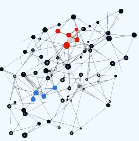
Fig 3. Visualization of selection of graph nodes in a Neighbor node loader
Consider the parameter num_neighbors = [4, 2] in the sampling configuration as illustrated below. For node 0, the first hop samples up to 4 neighbors (e.g., nodes 1, 2, 3, and 5). The second hop, starting from nodes 1 and 2, allows sampling up to 2 neighbors each—for instance, node 1 may connect to nodes 4 and 6.
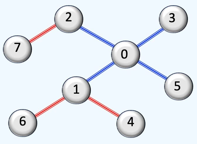
Fig. 3 Illustration of Neighbor Node Sampling with 2 hop [4, 2]
🔎 Hyperparameters Tuning Framework
We begin by encapsulating the hyperparameter optimization (HPO) process for the neighbor node sampler into a class named GNNTuning. The training parameters are initialized as a static dictionary that holds fixed hyperparameter values. Some entries, such as the loss function, are later updated dynamically once the data is loaded.
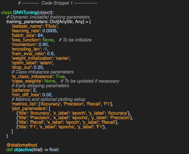
Some of the training parameters are arbitrary selected for the sake of this article. Practical applications may require a slightly different set of hyperparameters
⚠️ Optuna framework internal function are global therefore the method objective can only be implemented as a global function or static (or class) method.
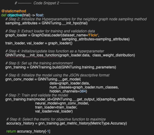
At the heart of the Optuna HPO process is the objective function, implemented as a static method. The following steps, centered around evaluating the target metric (accuracy in this case), are broadly applicable:
As previously described, training parameters are defined as static members of the GNNTuning class, with most values pre-initialized.
The objective function begins by setting the sampling-related attributes, which are the focus of the HPO.
It loads and extracts the training and validation data loaders based on the selected sampling strategy [ref 9].
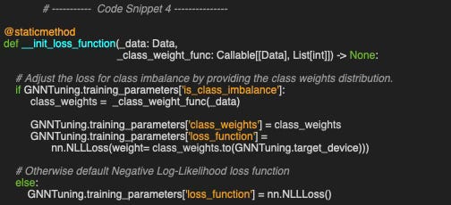
The loss function is updated dynamically if required given the dataset and need for compensating for class imbalance
The training-validation environment is then initialized.
The model is loaded from a descriptive JSON configuration.
Training and validation proceed using the candidate hyperparameters, while relevant metrics are collected.
Finally, the target metric—accuracy—is extracted and returned.
📌 Optuna library uses the term trial for hyperparameters configuration
The class GNNTraining wraps the execution of the generic training and validation methods and is described in a previous article, [ref 7].
📌 In our implementation, the final accuracy score is used as the objective to maximize. Alternatively, we could have chosen to optimize for precision, recall, or minimize the validation loss instead.
A key step in the process involves selecting the hyperparameters that maximize the previously defined objective. In this context, we focus on num_neighbors, which determines how many neighbors are sampled at each hop for a given node.
To work around Optuna’s limited support for multidimensional categorical values, we decomposed num_neighbors into two separate components:
The number of neighbors sampled at the first hop
The number of hops
A user-defined function, neighbor_sampling_func, then computes the number of neighbors for the second hop (n2), and for the third hop (n3), based on the initial count n1 from the first hop, as follows:
The categorical parameters are loaded to the trial in the __init_hpo method.
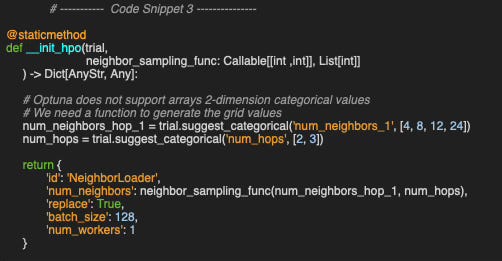
📌 Optuna does not natively support 2-dimensional categorical values (e.g., arrays of arrays) as categorical parameters. Optuna’s trial.suggest_categorical() is designed to work with a list of discrete scalar values — typically strings, numbers, or simple objects.
In our scenario, the loss function needs to be updated only in the case the classes or labels are associated with vastly different number of data instances as illustrated in the static method __init_loss_function.
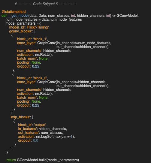
Lastly, we define the architecture and configuration of the Graph Convolutional Neural Network in the static method __get_model. It consists of two Graph Convolutional Blocks—each including a convolutional layer, an activation function, and dropout regularization—followed by a fully connected output block with a LogSoftmax activation
📈 Evaluation
Now it's time to put our hyperparameter optimization (HPO) setup into action. As shown in code snippet 6, we:
Choose the Tree-structured Parzen Estimator (TPE) as our Bayesian optimization strategy via TPESampler.
Set the optimization direction to maximize, since our objective is accuracy. (Note: if we were optimizing for validation loss, we would use the minimize direction instead.)
To reduce memory usage, we disable deep copy of each trial to avoid preserving its full state.

👉 The evaluation code available at geometriclearning/play/gnn_tuning_play.py
The two suggested trial values nun_neigbhors_hop_1 and num_hops in code snippet 3 generate the following combinations:
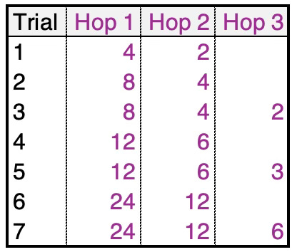
Table 1 Optuna trial configuration of distribution of number of sampled neighboring nodes
➡️ Optuna’s best trial is [24,12,6] for an accuracy 0.943
We display the 4 metrics, Accuracy, Precision, Recall and F1 as well as training and validation losses for a subset of these trials using 32 epochs.
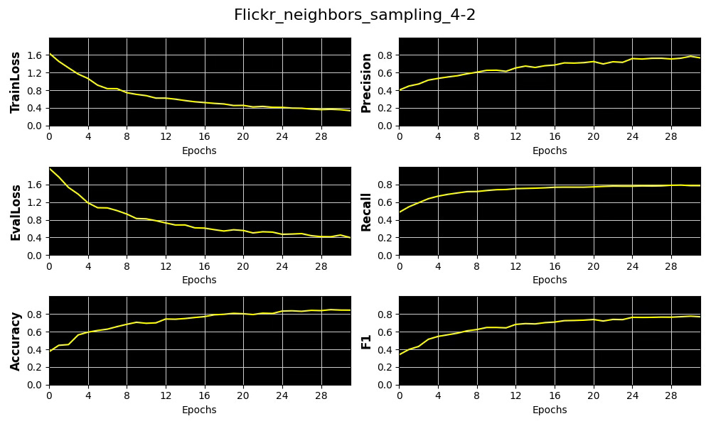
Fig. 4 Plots of 4 key metrics, training and validation loss for the distribution of number of sampled neighboring nodes per hop [4, 2]
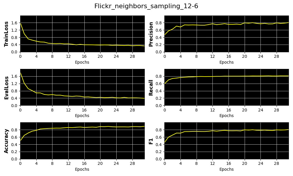
Fig. 5 Plots of 4 key metrics, training and validation loss for the distribution of number of sampled neighboring nodes per hop [12, 6]
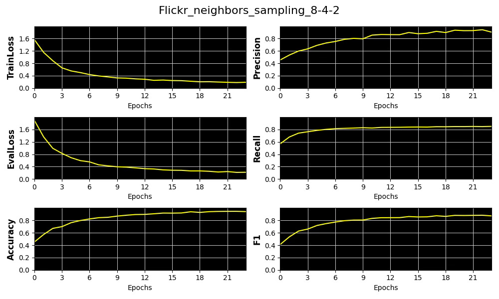
Fig. 6 Plots of 4 key metrics, training and validation loss for the distribution of number of sampled neighboring nodes per hop [8, 4, 2]
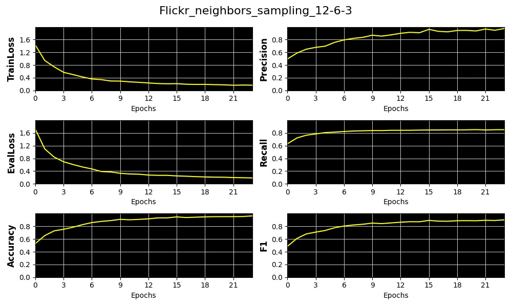
Fig. 7 Plots of 4 key metrics, training and validation loss for the distribution of number of sampled neighboring nodes per hop [12, 6, 3]
Finally, let’s compare the precision recall for the metrics for the 4 trial (hyperparameter configurations) displayed above.
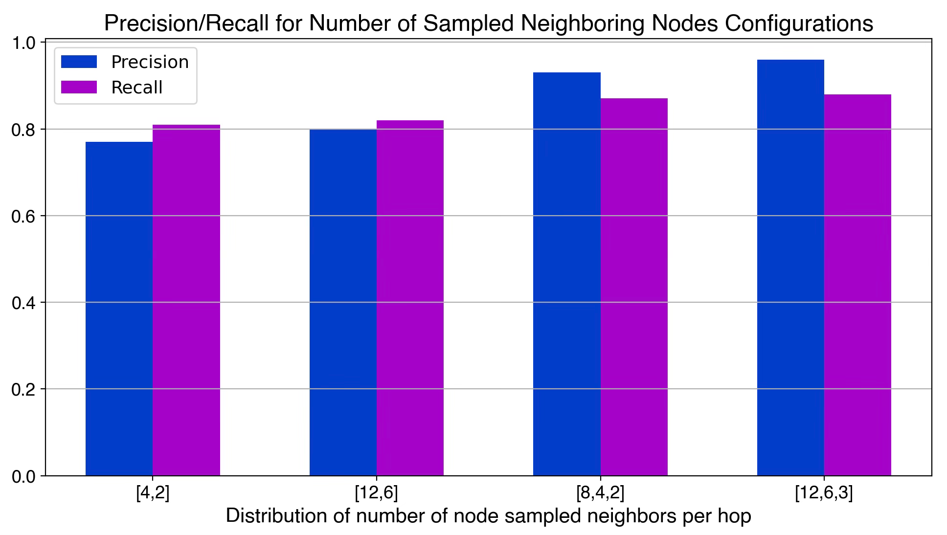
Fig. 8 Precision/Recall for a 4 distribution of number of sampled neighboring nodes per hop
⚠️ The computational overhead for training escalates sharply with the number of sampled nodes. In our case, using a [24, 12, 6] configuration results in a 23.4x increase in training time compared to a more lightweight [8, 4] setup.
🧠 Key Takeaways
✅ Manually tuning hyperparameters for complex models like Graph Neural Networks is often impractical.
✅ A more manageable approach is to decompose the search space into distinct categories—training parameters, model architecture, and sampling strategies.
✅ Optuna offers an intuitive and versatile solution for hyperparameter optimization across a wide range of scenarios.
✅ Its implementation of Bayesian Optimization via the Tree-structured Parzen Estimator (TPE) strikes an effective balance between performance and efficiency.
📘 References
Hyperparameter tuning - Geeks for Geeks
🛠️ Exercises
Q1 What are the two main categories of Bayesian Optimization?
Q2 Why is it advantageous to break down the hyperparameter search space into training parameters, model architecture, and node sampling methods?
Q3 Can you implement an __init_hpo method (referenced as code snippet 3) for the Graph Sampling Based Inductive Learning Method [ref 2]? As a reminder, the JSON string describing the sampling parameters is:
{
  'id': 'GraphSAINTRandomWalkSampler',
  'walk_length':3,
  'num_steps': 12,
  'sample_coverage': 100,
  'batch_size': 4096,
  'num_workers': 4
}
Q4 Can you modify the objective method (referenced as code snippet 2) so that it minimizes the validation loss?
Q5: Can you name one limitation of the Optuna hyperparameter optimization library?
👉 Answers
💬 News & Reviews
This section focuses on news and reviews of papers pertaining to geometric deep learning and its related disciplines.
Paper review: ReInc: Scaling Training of Dynamic Graph Neural Networks M. Guan, S. Singhal, T. Kim, A. Padmanabha Iyer - Georgia Institute of Technology = 2025
This paper presents an efficient and scalable approach to training Dynamic Graph Neural Networks (DGNNs) on very large datasets. The core idea is to reuse intermediate results and perform incremental aggregation (e.g., sum, average) to optimize computation.
DGNNs integrate a Graph Neural Network (GNN) for spatial encoding and a Recurrent Neural Network (RNN) for temporal encoding, making large-scale graph training computationally intensive. The GNN and RNN can be either stacked or integrated via RNN gates.
The primary objective of DGNNs is to predict future graph snapshots by leveraging both structural and temporal dependencies from a sequence of input snapshots, where each sequence represents an independent training sample. This follows a sequence-to-sequence framework using an encoder-decoder architecture, where the encoder generates hidden representations, and the decoder produces predictions through autoregression.
Scalability Strategy for Distributed Training:
To enhance scalability, the paper proposes a dynamic graph partitioning strategy alongside a three-pronged reusability mechanism:
Incremental aggregation to optimize computation.
Global and local caching of aggregations with a score-based eviction policy.
Graph placement (checkpointing) to reduce communication overhead.
The authors evaluate different DGNN variants on four graph datasets, demonstrating that DGNNs integrated via RNN gates outperform stacked DGNNs, achieving a cache hit rate of up to 52%.
Note: Neural Spacetimes (“https://arxiv.org/pdf/2408.13885”) can be utilized to integrate spatial and temporal embeddings for graph data.
Patrick Nicolas has over 25 years of experience in software and data engineering, architecture design and end-to-end deployment and support with extensive knowledge in machine learning.
He has been director of data engineering at Aideo Technologies since 2017 and he is the author of "Scala for Machine Learning", Packt Publishing ISBN 978-1-78712-238-3 and Geometric Learning in Python Newsletter on LinkedIn.