

Demystifying the Math of Geometric Deep Learning
Expertise Level ⭐⭐⭐⭐

Learn the essential mathematical concepts behind Geometric Deep Learning and world models without getting lost in equations - concepts only and no PhD required!
Applicability
Key Concepts
Discrete Differential Geometry
Abridged Glossary
🍩 Topology
Applicability
Key Concepts
Abridged Glossary
Applicability
Key Concepts
Abridged Glossary
Applicability
Key Concepts
Abridged Glossary
Applicability
Key Concepts
Abridged Glossary
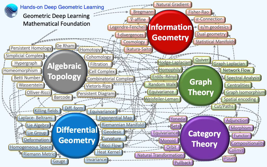
Geometric Deep Learning (GDL) has been introduced by M. Bronstein, J. Bruna, Y. LeCun, A. Szlam and P. Vandergheynst in 2017 [ref 1]. Readers can explore the topic further through a tutorial by M. Bronstein [ref 2, 3].
GDL is a branch of machine learning dedicated to extending deep learning techniques to non-Euclidean data structures. GDL offers a solution by enabling data scientists to grasp the true shape and distribution of data. An introduction to GDL is available in this newsletter [ref 4]
📌 As of early 2025, there is no universally agreed-upon, well defined scope for Geometric Deep Learning, as its interpretation varies slightly among authors.
This article surveys key mathematical ideas and assumes no prior expertise—don’t expect formal theorems or formulas. It distills the math specific to geometric deep learning from a sample of papers published between 2022 and 2024. The five-category breakdown (sections) is a pragmatic (and somewhat arbitrary) organizing choice. This article encompasses more topics than the strict mathematical foundation of GDL [ref 5].
⚠️ This article does not present topics such as topology or differential geometry from a rigorous mathematical standpoint. Rather, the subsequent sections are designed for data scientists and engineers navigating the theoretical foundations of geometric learning. We deliberately excluded the mathematical underpinnings of traditional and deep learning, including topics like linear algebra and differential calculus.
Each of the five sections answers three questions:
Applicability to ML: How do these mathematical methods support prediction, regression, and classification?
Key concepts: What are the essential mathematical ideas?
Abridged glossary: Which terms are used most often?
📌 Shared terminology: It is not uncommon that the same term is used across multiple fields with slightly different meaning. For instance, the strict definition of equivariance varies whether it is applied to topology, graphs or manifolds.
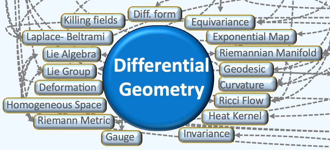
🌀 Differential Geometry
Differential geometry studies smooth spaces (manifolds) by doing calculus on them, using tools like tangent spaces, vector fields, and differential forms. It formalizes intrinsic notions such as curvature, geodesics, and connections—foundations for modern physics and for algorithms in graphics, robotics, and machine learning on curved data.
📌 I treat information geometry as distinct from differential geometry, much as I distinguish the natural gradient from the standard stochastic gradient. Other authors may differ.
Applicability
Differential geometry plays an important role in geometric deep learning and machine learning for Non-Euclidean spaces.
Stiefel/Grassmann groups for training on data manifold
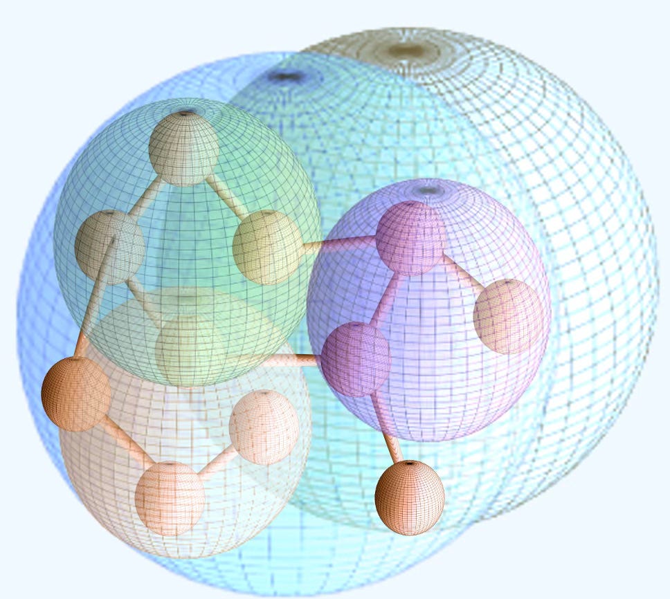
SO(3) Lie group & hyperbolic space for molecule embeddings on curved spaces.
Geodesics & parallel transport for gradient descent/ADAM optimizers for pose estimation and metric learning
Approximation of Laplace-Beltrami operator for learning on smooth manifolds for dimension reduction
Spectral clustering and heat-kernel for shape analysis and denoising
SE(3) Lie group and algebra for Robotics and 3D vision
Geodesic convolutions and gauge-equivariant mesh for climate data prediction
Wasserstein geometry for generative modeling and domain adaptation
Geometry of probability measures for class-imbalance
Diffeomorphic registration and Symmetric Positive Definite (SPD) groups on diffusion tensors for medical imaging
Ricci curvature and discrete Laplacian for anomaly and community detection
Heat kernel and Green’s function for Gaussian process on sphere
…
Key Concepts
Smooth Manifolds
Differential geometry is an extensive and intricate area that exceeds what can be covered in a single article or blog post. There are numerous outstanding publications, including book [ref 6], this newsletter [ref 7] and tutorials [ref 8, 9], that provide foundational knowledge in differential geometry and tensor calculus, catering to both beginners and experts
To refresh your memory, here are some fundamental elements of a manifold:
A manifold is a topological space that, around any given point, closely resembles Euclidean space. Specifically, an n-dimensional manifold is a topological space where each point is part of a neighborhood that is homeomorphic to an open subset of n-dimensional Euclidean space [ref 10]. Examples of manifolds include one-dimensional circles, two-dimensional planes and spheres, and the four-dimensional space-time used in general relativity.
Smooth or Differential manifolds are types of manifolds with a local differential structure, allowing for definitions of vector fields or tensors that create a global differential tangent space. A Riemannian manifold is a differential manifold that comes with a metric tensor, providing a way to measure distances and angles [ref 11]
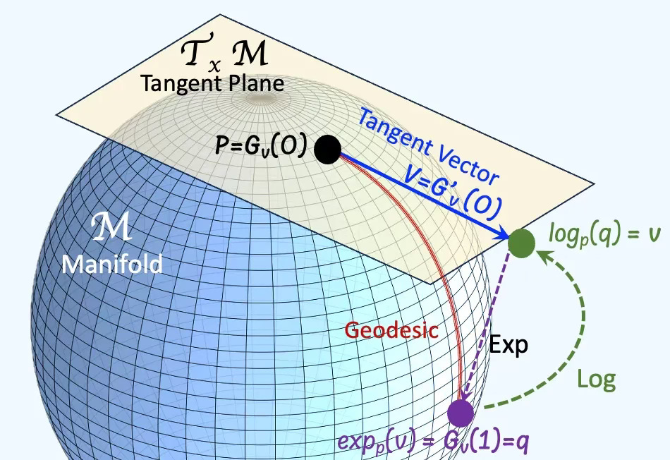
The tangent space at a point on a manifold is the set of tangent vectors at that point, like a line tangent to a circle or a plane tangent to a surface. Tangent vectors can act as directional derivatives, where you can apply specific formulas to characterize these derivatives [ref 12].
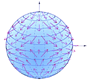
A vector field attaches a vector representing a direction and length at each point of a manifold. A Tensor field associates a tensor representing multi-dimensional values to each point on a manifold [ref 13].
A geodesic is the shortest path (arc) between two points in a Riemannian manifold. Practically, geodesics are curves on a surface that only turn as necessary to remain on the surface, without deviating sideways. They generalize the concept of a “straight line” from a plane to a surface, representing the shortest path between two points on that surface.
An exponential map turns an infinitesimal move on the tangent space into a finite move on the manifold. in simple terms, given a tangent vector, v the exponential map consists of following the geodesic in the direction of v for a unit of time.
A logarithm map brings a nearby point back to the tangent plane to define the tangent vector. It consists of finding the geodesic between two points on a manifold and extract is tangent vector.
Curvature measures the extent to which a geometric object like a curve strays from being straight or how a surface diverges from being flat. It can also be defined as a vector that incorporates both the direction and the magnitude of the curve’s deviation.
Intrinsic geometry involves studying objects, such as vectors, based on coordinates (or base vectors) intrinsic to the manifold’s point. For example, analyzing a two-dimensional vector on a three-dimensional sphere using the sphere’s own coordinates.
Extrinsic geometry studies objects relative to the ambient Euclidean space in which the manifold is situated, such as viewing a vector on a sphere’s surface in three-dimensional space.
Embedding: Extrinsic geometry examines how a lower-dimensional object, like a surface or curve, is situated within a higher-dimensional space.
Extrinsic Coordinates: These are coordinates that describe the position of points on the geometric object in the context of the larger space.
Normal Vectors: An important concept in extrinsic geometry is the normal vector, which is perpendicular to the surface at a given point. These vectors help in defining and analyzing the object’s orientation and curvature relative to the surrounding space.
Curvature: Extrinsic curvature measures how a surface bends within the larger space.
🤖 For math-minded readers
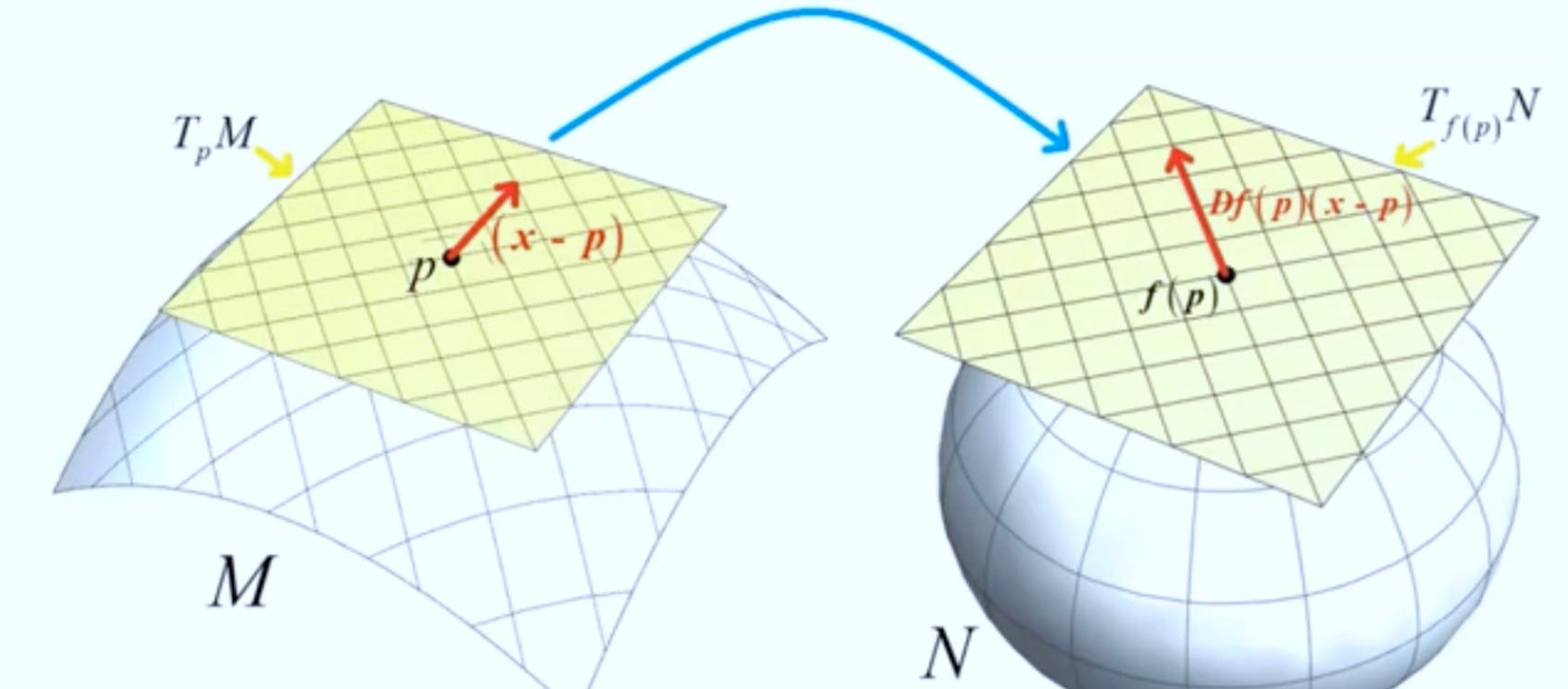
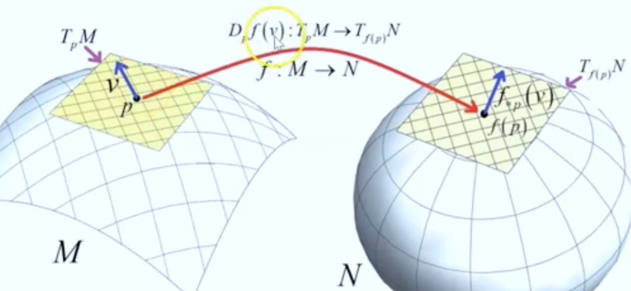
Given a smooth map F between two manifolds M and N, the pushforward move vector filed (directions & velocities) forward through F. Pushforward can be understood as follows: you stand at a point p∈M with a tiny arrow v showing which way you’re heading. Apply F: where and in what direction do you move in N? The pushforward dFp(v) is that new arrow at F(p). In layman terms, push forward pushed vectors.
Given a smooth map F between two manifolds M and N, the pullback brings metric back from N to M. The pullback describes how functions, gradients, differential forms or metrics on N manifold would be represented on M manifold. A simple description is that pullback pulls metrics.
📌 At its core differential geometry relies on traditional linear algebra, matrix operations and differential calculus [ref 14] which is omitted in this article.
Discrete Differential Geometry
Discrete Differential Geometry (DDG) is a field that translates the principles of smooth differential geometry—the study of curved shapes using calculus—into a language that computers can process, primarily using meshes and polygons.The core elements of this field are categorized by how they discretize the geometry of shapes and the operators that act upon them.
Rather than dealing with infinite, smooth surfaces, DDG uses combinatorial structures to represent geometry such as Simplicial Complexes, Cell Complex, Hypergraphs or meshes.
Ollivier-Ricci curvature applies the Ricci curvature of Riemannian smooth manifold to graphs and simplicial complexes [ref 43].. The Ollivier-Ricci Curvature (ORC) serves as a discrete approximation that uncovers local topology and geometric properties through the lens of optimal transport, commonly used in Information. Geometry.
Differential Operators
The covariant derivative measures the rate of change of vector fields, considering the variation of basis vectors. For instance, in flat space, the covariant derivative of a vector field corresponds to the ordinary derivative, calculating both the derivative of the vector components ui and the derivative of the basis vectors.
The covariant derivative is often conceptualized as an affine connection because it links the tangent spaces (or planes) at two points on the manifold. Parallel transport involves moving a geometric vector or tensor along smooth curves within the manifold. This process is facilitated by the covariant derivative, which enables the transportation of manifold vectors along these curves, ensuring they remain parallel according to the connection.
The Levi-Civita connection is a type of metric connection that is compatible with the metric tensor of a Riemannian manifold. Its covariant derivative of the metric tensor with respect to the Levi-Civita connection is zero. The property of parallel transport ensures that the connection preserves the inner product structure defined by the metric tensor.
The gradient transforms a scalar field into a vector field.
Divergence is a vector operator used to quantify the strength of a vector field’s source or sink at a specific point, producing a signed scalar value.
The curl operator represents the minute rotational movement of a vector in three-dimensional space. This rotation’s direction follows the right-hand rule (aligned with the axis of rotation), while its magnitude is defined by the extent of the rotation
In mathematics, the Laplacian, or Laplace operator, is a differential operator derived from the divergence of the gradient of a scalar function in Euclidean space
A differential form is a smooth, coordinate-free integrand for curves, surfaces, and higher-dimensional sheets. At each point of a space (manifold) it assigns an antisymmetric multilinear “measuring rule” that eats k tangent vectors and returns a number. A k-form is what you integrate over k-dimensional objects: 0-form is smooth function as integration over data points. 1-form is an integration along a curve and a 2-form is an integration over a surface.
Lie groups & Algebras
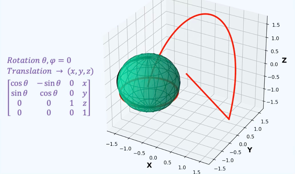
Lie groups play a crucial role in Geometric Deep Learning by modeling symmetries such as rotation, translation, and scaling. This enables non-linear models to generalize effectively for tasks like object detection and transformations in generative models. The Special Euclidean Group [ref 15] and Special Orthogonal Group [ref 16] are two examples of Lie groups.
In differential geometry, a Lie group is a mathematical structure that combines the properties of both a group and a smooth manifold. It allows for the application of both algebraic and geometric techniques [ref 17]. As a group, it has an operation (like multiplication) that satisfies 4 axioms:
Closure
Associativity
Identity
Invertibility
A Lie algebra is a mathematical structure that describes the infinitesimal symmetries of continuous transformation groups, such as Lie groups. It consists of a vector space equipped with a special operation called the Lie bracket, which encodes the algebraic structure of small transformations. Intuitively, a Lie algebra is a tangent space of a Lie group [ref 17].
Symmetric & Symplectic Spaces
A symmetric space is uniform as every point looks the same as every other, and around each point. It is equipped with a metric. If you walk along any geodesic through the point, the space has an isometry that reverses your direction but keeps the point fixed—like reflecting across that point and therefore the distances are not changed. Sphere (positive curvature) - 2D space (zero curvature) or hyperbolic plane (negative curvature). Symmetric spaces are critical in statistics, signal processing and non-Euclidean machine learning [ref 18].
A symplectic space (or symplective manifold) is a smooth space equipped with a metric (length or angle) or have curvature but relies on areas (e.g., parallelogram) or volume (e.g., tetrahedron). Transformations over a Symplective space preserve areas/volumes. Symplectic spaces are related to simplicial complex and describes global geometric properties [ref 19].
Abridged Glossary - 1
Deformation (scaling, stretching, bending,….): A signal defined on a geometric domain (like a graph, manifold, or group) changes under transformations of that domain.
Deformation stability: A model’s ability to remain robust to small, non-structured distortions in the input in the context of equivariance
Diffusion on manifolds: Models designed for data constrained to lie on spheres, Lie groups, or statistical manifolds.
Directional derivative: Measures a function change as you move in a specific direction.
Domain deformation: A transformation or distortion of the geometric structure (domain) on which signals are defined.
Equivariant neural network: A network that respects the symmetries of the input data.
Exponential map: A map from a subset of a tangent space of a Riemannian manifold.
Flow matching: A generative modeling technique is to learn a transformation (or flow) that maps a simple base distribution (like a Gaussian) to a complex target distribution.
Gauge: A local choice of frames or coordinates used to describe geometric objects, particularly when those objects are defined on fiber bundles.
Geodesics: Curves on a surface that only turn as necessary to remain on the surface, without deviating sideways.
Heat kernel: Solution to the heat equation with appropriate boundary conditions. It is used in the spectrum analysis of the Laplace operator.
Homogeneous space: A manifold on which a Lie group acts transitively.
Killing field: A vector field on a pseudo-Riemannian manifold that preserves the metric tensor. The Lie derivative with respect of the field is null.
Laplace-Beltrami operator: Operator using second order derivative to quantify the curvature in a data manifold using a Riemannian metric.
Lie algebra: A vector space over a base field along with an operation locally called the bracket or commutator that satisfy bilinearity, Anti-symmetry and Jacobi Identity.
Lie-equivariant networks: Neural networks that are equivariant to transformations from a Lie group, such as rotations, translations, scaling, or Lorentz transformations.
Lie group: A differentiable space that is itself a group, meaning it supports smooth multiplication and inversion.
Logarithm map: A fundamental tool that translates points on a manifold back to the tangent space at a base point, typically to linearize the geometry for computation or analysis.
Manifold: A topological space that, around any given point, closely resembles Euclidean space.
Neural operators: A class of machine learning models that learn mappings between infinite-dimensional function spaces.
Point cloud: A fundamental representation for real-world 3D data, especially when acquired via sensors.
Quantum groups: Mathematical structures that generalize Lie groups and Lie algebras, particularly in the context of non-commutative geometry and quantum physics.
Ricci curvature: A measure of how much the geometry of a manifold deviates from ‘being flat’, focusing on how volume or distance between geodesics changes.
Riemannian manifold: A differential manifold that comes with a metric tensor, providing a way to measure distances and angles
Riemannian metric: Assigns to each point a positive-definite symmetric bilinear form (e.g. dot product) to a manifold in a smooth way. This is a special case of metric tensor.
Smooth or Differentiable manifold: A type of manifolds with a local differential structure, allowing for definitions of vector fields or tensors that create a global differential tangent space.
Spectral convolution: Transformation of a signal into the frequency domain using the Laplacian eigenfunction basis, applying a spectral filter (pointwise multiplication), and transforming back.
Stratified space: A space decomposed into smooth manifolds (called strata) arranged in a partially ordered fashion.
Tangent space at a point on a manifold: A set of tangent vectors at that point, like a line tangent to a circle or a plane tangent to a surface.
Von Mises-Fisher: A uniform random generator distributes data evenly across the hypersphere, making it unsuitable for evaluating k-Means.
🍩 Topology
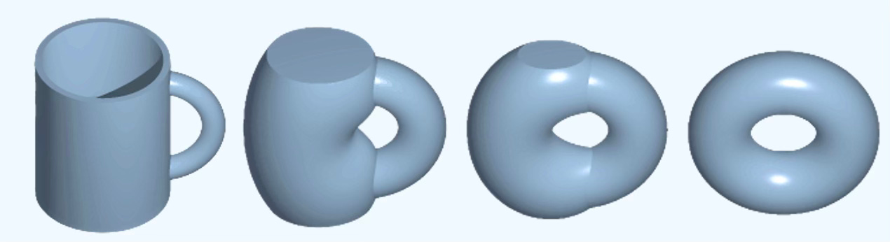
Topology describes shape properties unchanged by continuous deformations, provided no holes are opened or closed and no tearing or gluing occurs.
Applicability
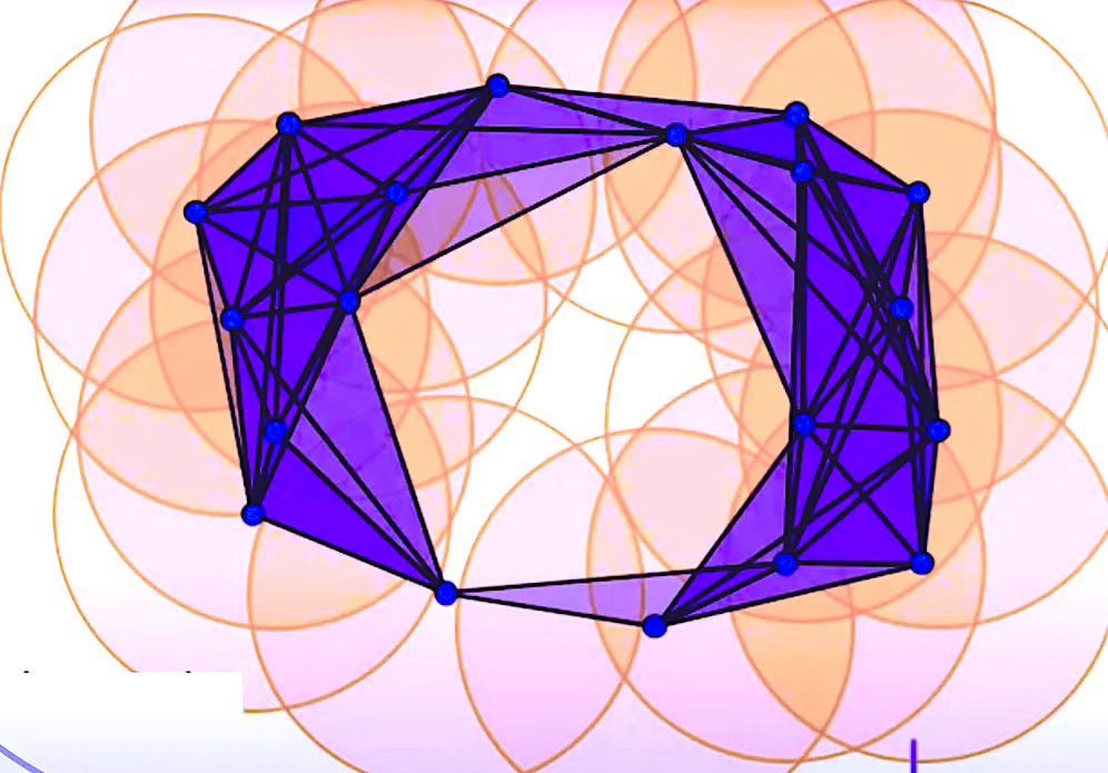
Topology gives shape-aware summaries (holes, connectivity, loops) that are stable to noise and invariant to many deformations.
Here are some of the applications of topological features
Filtrations such as alpha-complex, cubical and Vietoris-Rips are applicable to point clouds and embeddings for 3D medical volumes
H-invariants such as H0 (components), H1 (rings) and H2 (voids) support persistence entropy and therefore dimension reduction for shape, molecules and regime change in time series.
Vectorization supplements existing kernel methods for anomaly detection and community clustering
Topology-aware regularizers improves robustness against adversarial noise
Hole penalizing factor can be added to loss function for training and inference
Differentiable persistence and Betti numbers for back-propagation (training)
Simplicial/Cell/Combinatorial complex networks using Hodge Laplacians to capture geometric attributes such as flows, cavities or curls.
Hodge Graph Neural Network learning k-forms for representation of meshes and traffic flows.
Mappers for data exploration and visualization
Topological change-point and sliding-window embedding with persistent homology for regime changes vs. periodicity
Homology of latent spaces for auto-encoders
Graph filtrations for clique complex
…
Key Concepts
Foundation
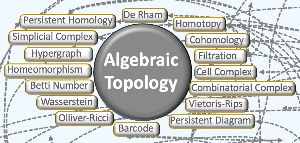
General Topology and Algebraic Topology in particular are the foundation of Topological Deep Learning [ref 20].
Point-set (general) topology treats the foundational definitions and constructions of topology. Key concepts include continuity (pre-images of open sets are open), compactness (every open cover admits a finite subcover), and connectedness (no separation into two disjoint nonempty open subsets) [ref 21].
A topological space is a set equipped with a topology—a collection of open sets (or neighborhood system) satisfying axioms that capture “closeness” without distances. It may or may not arise from a metric. Common examples include Euclidean spaces, metric spaces, and manifolds.
Homeomorphism or topological equivalence is defined as a bijective, continuous map with continuous inverse between two spaces that are considered similar. Algebraic topology seeks invariants that do not change under such equivalences.
Homotopy
Homotopy theory is a branch of algebraic topology that studies the properties of spaces that are preserved under continuous deformations, called homotopies. It helps in distinguishing spaces that are topologically the same from those that are not and offers tools for working with complex spaces in mathematics and applied sciences [ref 22]. Two mappings or spaces are homotopic if one can be deformed continuously into the other. Homotopy equivalence is analogous to a parameterized family of mappings and is weaker than topological equivalence.
The loop space of a topological space is the space of all loops within that space based at a point, and its Homotopy groups capture the space’s properties
A Fundamental group is an algebraic group that is topological invariant of the space to which it is associated. loops based at a point are classified up to deformation, with loop concatenation giving a group. For example, maps from higher-dimensional spheres generalize the fundamental group.
The Betti number is a key topological invariant that count the number of certain types of topological features in a space. It provides a concise summary of the space’s shape and structure, especially when dealing with high-dimensional or complex datasets (dimension 0: Connected components, dimension 1: holes, loops, dimension 2: 3D holes and voids,)
Topological Complexes
There are 4 key topological domains [ref 23]
Simplicial complexes
Cellular complexes
Hypergraphs
Combinatorial complexes
A Simplicial Complex is a generalization of graphs that model higher-order relationships among data elements—not just pairwise (edges), but also triplets, quadruplets, and beyond (0-simplex: node, 1-simplex: edge, 2-simplex: Triangle, 3-simplex: Tetrahedron, ) [ref 24].
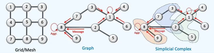
A Cellular (or CW, Cell) Complex is a topological space obtained as a disjoint union of topological disks (cells), with each of these cells being homeomorphic to the interior of a Euclidean ball. It is a general and flexible structure used to build topological spaces from basic building blocks called cells, which can be points, lines, disks, and higher-dimensional analogs.
A Hypergraph is the extension of the traditional graph where edges (called hyperedges) can connect any number of nodes, not just two. While edge of a graph models a binary relationship, a hypergraph models higher-order relationship among group of nodes
Combinatorial Complex are structured collections of simple building blocks (like vertices, edges, triangles, etc.) that models the shape of data in a way that is amenable to algebraic and computational analysis. These topological domains are built from data into a nested sequence known as Filtration. Each domain includes the previous one and represents the data’s topology at a certain scale or resolution.
Cochains are signal or function that map, known as Cochain Map a combinatorial complex of rank k to a real vector. Cochains defines the Cochain Space. The Cochain Map uses incidence matrix as transformation. An Incidence Matrix is an encoding of relationship between a k-dimensional and (k-1) -dimensional simplices (nodes, edges, triangle, tetrahedron,..) in a simplicial complex.
Homology & Cohomology
Homology/Persistent Homology decomposes topological spaces into formal chains of pieces. Numerical summaries such as Betti numbers and the Euler characteristic arises from these chains to count higher-order structural features such as loops, holes, cavities/voids [ref 25]. A barcode represents the appearance/disappearance of these structure features (topological elements) given a radius.
An Abelian (commutative) group is a group whose operation is commutative. Common sources include any vector space under addition, rings and fields under addition, and the multiplicative group of a field (nonzero elements).
Chain complex is a sequence of abelian groups ⋯- d(n+1) → C(n) — d(n)→ C(n-1) —d(n-1)→ … with boundary maps satisfying d(n−1)∘d(n)=0. Cochain complex: the “opposite-direction” version ⋯- d(n-1) → C(n) — d(n)→ C(n+1) —d(n+1)→ … with d(n+1)∘d(n)=0; this duality mirrors covariant vs. contravariant behavior [ref 26].
A Cohomology from a cochain complex gives algebraic invariants of a space. Compared to homology, cohomology often carries additional structure (e.g., a graded-commutative ring via the cup product) and many versions arise by dualizing homology constructions.
De Rham Cohomology measures the “holes” of a smooth manifold using differential forms. Two forms count as the same cohomology class if they differ by a derivative (an exact form) [ref 27]. Forms whose derivative is zero are closed.
Filtrations of a space across scales give rise to persistent homology, summarizing the birth and death of features; distances between summaries are stable under small perturbations.
A sheaf is a way to attach information to every open region of a space (a map, a surface, a network), and to make sure those pieces of information fit together consistently [ref 28]. Mathematically, A sheaf on a geometrical structure S valued in a target category V is a rule D, which associates, with any element s P S an objection D(s) of V and any morphism D(e): D(s1) → D(s2) for any arrow s1 → s2. A collection of sheaves constitutes a Category. A Sheaf Diffusion on D is a dynamical system which brings an arbitrary state of the medium to an equilibrium state.
A partially ordered set (poset) is a set S together with a binary relation ď, called the (non-strict) partial order, which satisfies:
s <= s for any s in S
s1 <= s2 and s2 <= s3 imply s1<= s3
s1 >= s2 and s2 >=s1 imply s1== s2.
A symplectic manifold is a smooth space (M,ω) of even dimension 2n equipped with a 2-form ω that is Closed (dω=0) and non-degenerate: the map v ↦ ιvω sends each tangent vector v to a unique covector.
Decision topology is the topology of a classifier’s decision regions and boundaries—how many pieces they have and how they connect—used to quantify boundary complexity, robustness, and generalization.
Abridged Glossary - 2
Barcode: A multi-set of intervals that records when topological features appear and disappear along a filtration in persistent homology.
Betti number: distinction of topological spaces based on the connectivity of n-dimensional simplicial complexes
Cellular complex: A space built by gluing together basic building blocks called cells that objects homeomorphic to open shapes such as polygons, solids..
Chain map: A map between chain complexes of modules is a sequence of module homomorphisms
Cohomology: A way to measure the global shape of a space using functions on elements rather than the elements themselves.
Combinatorial complex: Encode arbitrary set-like relations between collections of abstract entities. It permits the construction of hierarchical higher-order relations, analogous to those found in simplicial and cell complexes
De Rham cohomology: Cohomology of complex of differential forms (smooth manifolds)
Filtration: A nested family of spaces indexed by a parameter so that earlier sets are contained in later ones. It is a sequence of subcomplexes for finite simplicial complex
Homeomorphism: A bijective map between topological spaces that is continuous and whose inverse is also continuous
Hypergraph: Graph that supports arbitrary set-type relations without the notion of ranking.
Homotopy: Ability for two continuous maps can be deformed into each other without tearing.
Olliver-Ricci curvature: A notion of (coarse) Ricci curvature defined on any metric measure space using optimal transport. It is a key concept in discrete manifolds.
Persistent homology: Tracks topological features across different scales. It captures higher-order structural features such as holes, cycles and cavities
Persistent diagram: An alternative to visualize persistence homology. It is a summary of how topological features appear and disappear across a filtration.
Simplicial complex: A structured set of simplices (points, edges, triangles, and their n-dimensional analogues) in which every face of a simplex and every intersection of simplices is itself included.
Vietoris-Rips complex: A simplicial complex built from a metric space such as a point cloud using a distance threshold. It is analogous to a clique complex.
Wasserstein distance: An optimal transport metric that measures how much work it takes to match the multiset of birth–death points from one persistent diagram to those of another.
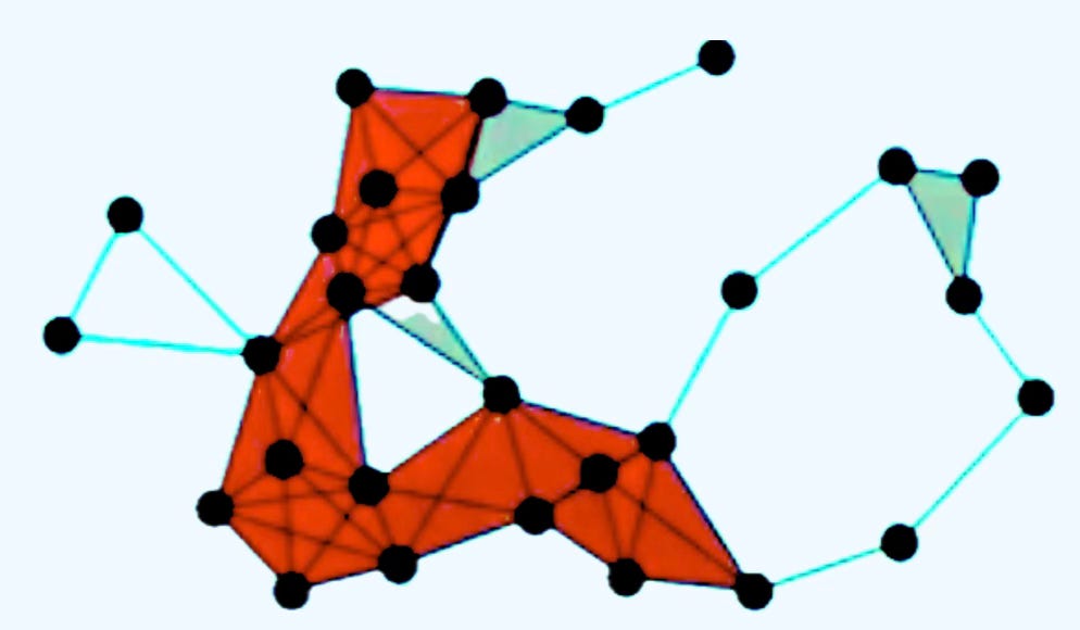
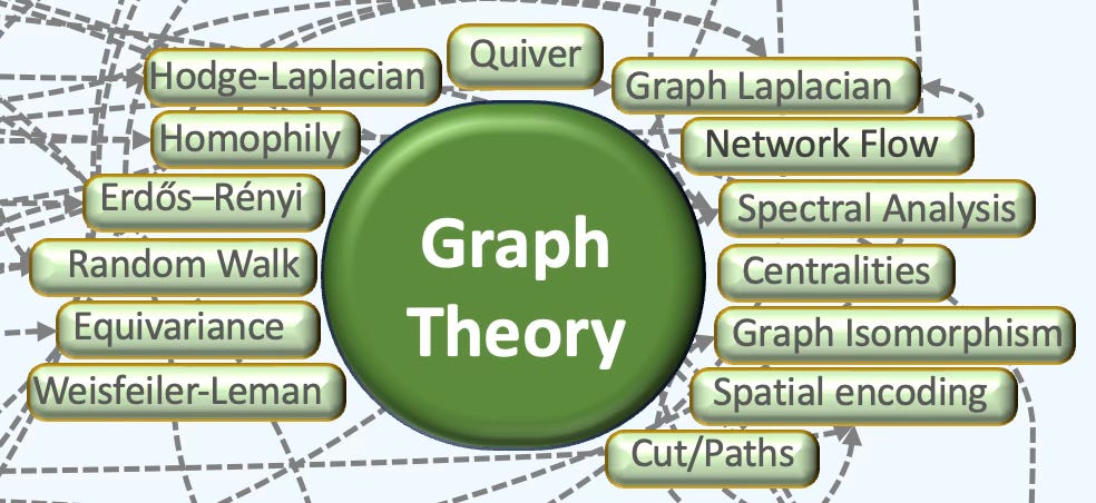
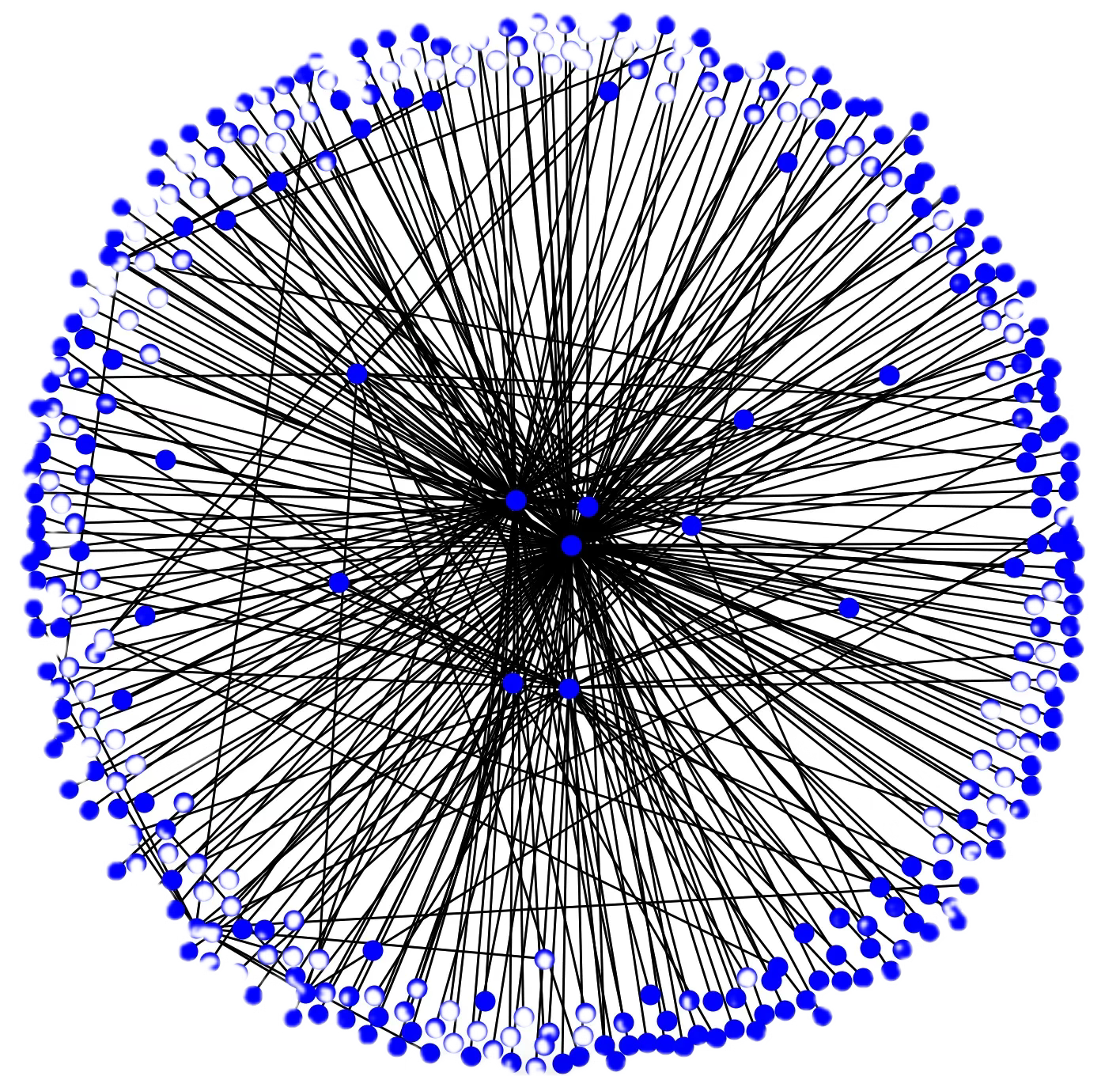
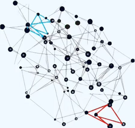
🔗 Graph Theory
Graph theory concerns mathematical graphs used to encode pairwise relations. A graph comprises vertices and edges; a digraph differs from an undirected graph in that each edge is oriented.
Applicability
Graph encoding for Node classification, link prediction, graph classification/regression/recommendations
Graph embeddings to reduce dimension of node/graph feature vector for downstream classification or regression tasks
Spectral clustering on graph structures to detect communities
Message passing for probabilistic graphical models such as Markov chains, Bayesian networks
Causal networks to enhance variational inference
Spatiotemporal representation for graph Transformers
Subgraphs with Ricci flow and centrality/curvature for anomaly and fraud detection
Graph cuts to enhance image segmentation and point cloud processing
Label propagation over similarity graphs to improve node classification
Routing, matching & scheduling algorithm for optimization
…
Key Concepts
Definitions
Graph theory studies networks made of nodes/vertices and links/edges—who’s connected to whom, and what that structure implies.
I recommend the text book Graph theory from Schaum as it includes step by step examples and exercises [ref 29].
A graph can be [ref 30]
fixed or dynamic/temporal
undirected or directed
weighted or unweighted
a simple graph, a multigraph or a hypergraph
📌 The terms node and vertex are used interchangeably in this newsletter.
A directed acyclic graph (DAG) is a directed graph with no cycles—following the arrow directions never brings you back to where you started. A graph is bipartite if its vertices can be partitioned into two independent sets U and V; every edge joins a vertex in U to one in V. A graph without loop is a multigraph [ref 30]. A complete graph is a graph in which there is exactly one edge joining every pair of vertices/nodes. A planar graph is a graph represented in a plane such that two edges of the graph intersect except at a vertex to which they are both incident. A hypergraph is a generalization of a graph: Any edge can join any number of vertices [ref 31].
Algorithms
Typical graph descriptors include paths, cycles (including loops), distances, in/out degrees, and centrality indices such as betweenness, closeness, and density. Standard representations are the adjacency matrix, the edge list (source–target pairs), and the adjacency list (node with its neighbor set). The homophily factor assesses similarity between a node (or edge) and its neighborhood.
🤖 For math-minded readers
Two graphs G & G’ are isomorphic is there is one-to-one correspondence, known as an isomorphism f: G → G’ such there is an edge between f(v) & f(w) if and only if there is an edge between v & w.
Common problems in graph theory include:
Traversal: breadth-first (from a given node explores all neighboring nodes/vertices first then to moving on the each of their respective neighbors) and depth-first search (from any given node, walks as far as possible along each path/sequence of edges before backtracking).
Shortest paths: Dijkstra’s (traversal of weighted graph from any given node) or Bellman–Ford algorithms (traversal of weighted digraph for which weight can be negative).
Heuristic search / routing/best search: A* (and variants) for layout or path optimization (shortest path from any given node to any other node by minimizing the cost of the path)
Maximum flow: Finding a path through a network that produces the maximum possible flow rate.
Min-cut (partitioning): Computing min-cuts is partitioning the nodes/vertices of a graph into two disjoint subsets/subgraphs that minimizes some metric or distance.
Minimum spanning tree: A sequence of edges of an undirected graph without cycles that minimize sum of the weights of the edges in the path.
Coloring: A simpler variant of graph labeling that colors nodes such no two adjacent nodes share the same color.
Clique extraction: Extraction of the nodes sharing given properties or features. A node can belong to multiple cliques. Edges in a clique are quite often characterized with high density while edges across cliques exhibit low density.
Community detection/graph clustering. Task of partitioning a social graph into groups of individuals. It is regarded as a special case of clique extraction. It leverages spectral clustering techniques such Laplacian eigenvectors or random walks.
Embeddings: learning/constructing graph embeddings.
Random graphs: generating models like Erdős–Rényi.
Power-law model: Random graph whose degree distribution follows the power law
Percolation on graphs: Random deletion of nodes or edges while preserving graph connectivity.
…
Spectral Properties
Linear algebra is used to extract spectral properties such as Laplacian, eigenvalues and eigenvectors, algebraic connectivity. Heat kernels are used for random walks and diffusion.
Spectral graph theory studies how a graph’s structure is reflected in the eigenvalues and eigenvectors of its associated matrices—especially the adjacency and (normalized) Laplacian. The spectrum (the multiset of eigenvalues) is invariant under graph isomorphisms. Spectral decomposition expresses a diagonalizable graph matrix as (UDU⊤ for symmetric cases), separating eigenvalues and eigenvectors [ref 32].
Spectral properties of a graph can be represented as matrices:
Degree matrix D: diagonal matrix with Dii=deg(i) (number of edges incident to node i).
Adjacency matrix A: Aij=1 if nodes i and j are adjacent, else 0. For simple graphs, the diagonal is 0.
Incidence matrix B: rows = vertices, columns = edges.
Undirected: Bv,e=1 if vertex v is incident to edge e, else 0 (many texts instead use ±1 with an arbitrary orientation).
Directed: Bv,e=−1 if e leaves v, +1 if e enters v, else 00.
Laplacian L: L=D−A. For an unweighted undirected graph, Lii=deg(i) and Lij=−1when i∼j, else 0 (symmetric, PSD). For directed graphs, several variants exist (out-/in-/symmetrized).
Higher-order: Up-, Down-, and Hodge–Laplacians built from incidence matrices are fundamental in simplicial and combinatorial topology.
…
Coloring
The Weisfeiler–Lehman (WL) algorithm is a combinatorial test for graph isomorphism and a standard yardstick for Graph Neural Networks’ expressiveness. It generalizes color refinement by operating on k-tuples of nodes: higher k captures richer relational structure and distinguishes more graphs [ref 33].
1-WL: refines colors using node neighborhoods (nodes/edges).
2-WL: refines colors on pairs of nodes (captures pairwise patterns).
3-WL: extends to triples of nodes.
…
k-WL: operates on k-tuples; expressiveness increases with k
∞-WL: the most expressive WL variant; theoretically powerful but computationally heavy.
In graph learning theory, WL is widely used to analyze when two graphs are distinguishable by structure and to benchmark the expressiveness of Graph Neural Network architectures.
📌 Graphs algorithms rely on matrix operations [ref 34] which are omitted in this article.
Abridged Glossary - 3
Centrality: Number or rankings of nodes within a graph that corresponds to their position. The list of types of centrality includes betweenness centrality, eigenvector centrality, degree centrality, closeness centrality and page rank.
Equivariance: A form of symmetry for functions from one graph with symmetry to another graph.
Erdős–Rényi: Model for which all graphs on a fixed vertex set with a fixed number of edges are equally likely
Graph cut: A partition of the vertices of a graph into two disjoint subsets.
Graph isomorphism: A bijection between the vertex sets of two graphs. This is an equivalence relation used to categorize graphs.
Graph Laplacian: An operator in spectral graph theory that encodes the structure of a graph and is widely used in graph neural networks.
Graph path: A path in a graph is a finite or infinite sequence of edges which joins a sequence of vertices which are all distinct.
Hodge–Laplacian: Canonical Laplace operator on differential k-forms on a Riemannian manifold.
Homophily: Property for which nodes with the same label or attributes are more likely to be connected in the network.
Network flow: A graph with numerical capabilities on its edges
Network flow problem: Types of numerical problem in which the input is a flow defined as numerical values on a graph edges.
Quiver: A directed graph where loops and multiple arrows between two vertices are allowed.
Random walk: A stochastic process that describes a path that consists of a succession of random steps on a graph.
Set (a.k.a. category Set). A category with sets as object and function between sets as morphisms.
Spatial encoding: Spatial information such as related to curvature used as features of node or edges.
Spectral analysis: Study of the properties of a graph in relationship to its adjacency matrix and Laplacian matrix
Weisfeiler-Lehman: A graph test for the existence of an isomorphism between two graphs as a generalization of the color refinement algorithm.
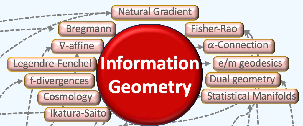
🧭 Information Geometry
Information geometry applies differential-geometric tools to probability and statistics. It treats families of distributions as statistical manifolds—Riemannian manifolds whose points are probability laws—often equipped with a pair of conjugate affine connections; in many cases these structures are dually flat.
Applicability
Supporting statistical manifolds with Fisher-Rao metric
Natural gradient to improve stability during model training
Support for variational inference using dual geometry
Leveraging exponential families to reinforcement learning
Key Concepts
Basics
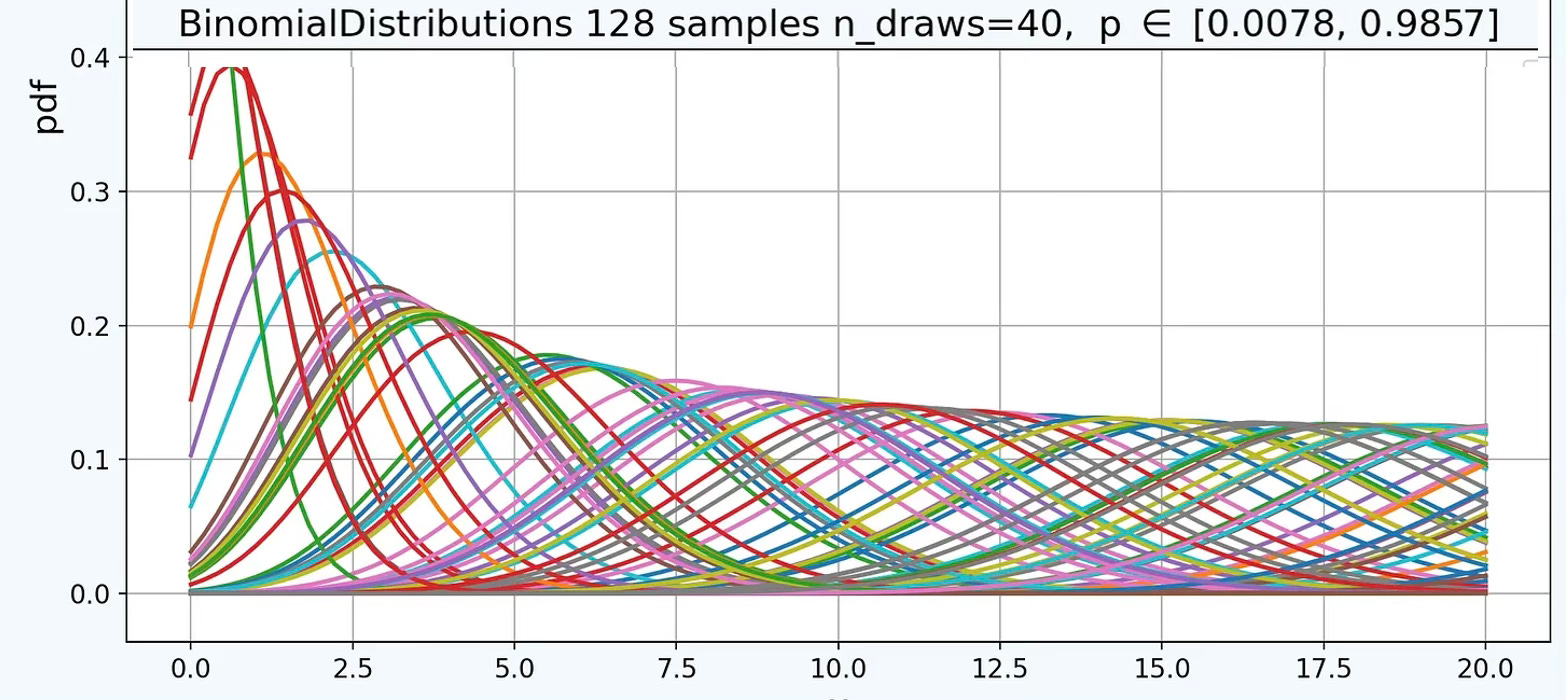
Information Geometry is derived from mathematical statistics and information theory. The well-known field of statistics covers discrete probability variables such as Binomial or Poisson distributions and probability density continuous functions such as Exponential or Gaussian distribution. Information theory pioneered by Claude Shannon owed its origin to thermodynamics and concern with the quantization of Entropy as a measure of the disorder (or chaos) in an irreversible system [ref 35, 36]. The Gamma distribution plays a pivotal role in information theory.
Statistical Manifolds
Information geometry leverages Riemannian manifolds and metric, parallel transport, connection, tangent spaces, curvature and geodesics to extract geometric properties of various families of probability density functions.
Statistical manifolds are smooth families of probability distributions represented as geometric, parameterized spaces. The canonical Riemannian metric related to the distribution parameters is known as the Fisher-Rao metric or Fisher Information Matrix [ref 37, 38]. Alongside of the Fisher-Rao metric, information geometry equips the manifold with two α-connections, known as dual affine connections: e-connection and m-connection. Parameters of exponential distributions are affine e-connections while expectation parameters are affine m-connection. Statistical manifolds can be induced with a Hessian metric for exponential distribution.
The steepest descent under the Fisher-Rao metric is defined as the natural gradient, under which Expectation-Maximization and variational inference are e or m-projections with Kullback-Leibler divergence.
Optimal Transport (OT) provides a way to define distances between probability distributions by considering the underlying geometry of the space those distributions live on. While traditional Information Geometry (Fisher-Rao) focuses on how distributions change relative to each other purely as “statistical points,” Optimal Transport focuses on the physical effort required to move “mass” from one distribution to another.
Non-Exponential Distributions
Information Geometry applies to Bivariate family of probability distribution such as McKay Bivariate Gamma and LogGamma manifold, Freund Bivariate Exponential and LogExponential manifold and Bivariate Gaussian manifold.
Information geometry extends spatial stochastic (Poisson) processes
Divergences
Kullback–Leibler (KL) divergence—a.k.a. relative entropy—measures how one probability distribution departs from a reference/target distribution. It’s not a metric (it’s asymmetric and fails the triangle inequality).
Jensen–Shannon (JS) divergence—the symmetrized, KL-based measure—quantifies similarity between two distributions and has a closed form for Gaussian families.
Bregman divergence (or Bregman “distance”) is a difference measure generated by a strictly convex function. When points represent probability distributions (e.g., model parameters or datasets), it serves as a statistical divergence. A basic example is squared Euclidean distance.
Abridged Glossary - 4
α-connections: Dual pair of affine connection on a statistical manifold such as exponential family, with respect of the Fisher-Rao metric. Amari -1 connection is referred as m-connection and +1 connection as e-connection.
α-divergence: A particular type of f-divergence related to dual connection
∇-affine coordinates: Affine e-connection or m-connection in which a local charts has null Christoffel symbols and geodesics are straight lines.
Bregman divergences: A class of distance-like functions that generalize the squared Euclidean distance using a convex function.
Dual geometry: Pair of connection and conjugate connection related to dually flat manifolds.
e/m geodesic: Curves on e-connection or m-connection which coordinates are linear along the geodesic.
f-divergences: A large family of statistical distance between probability distribution defined from a convex function. Kullback-Leibler and Jensen-Shannon are the most well-known statistical distances.
Fisher–Rao metric (also referred as the Fisher information matrix): A Riemannian metric defined on a statistical manifold, which is a smooth space where each point corresponds to a probability distribution.
Itakura-Saito divergence: A measure of the difference between a Spectrum (frequency) and its approximation. This is a type of Bregman divergence.
Legendre-Fenchel transformation: Generalization of the Legendre transformation to affine spaces that defines a convex conjugate.
Natural gradient, NG: An optimization method that adapts the standard gradient by accounting for the geometry of the parameter space representing probability distributions.
Statistical manifold: Smooth manifolds in which each point represents a probability distribution, parameterized by one or more variables.
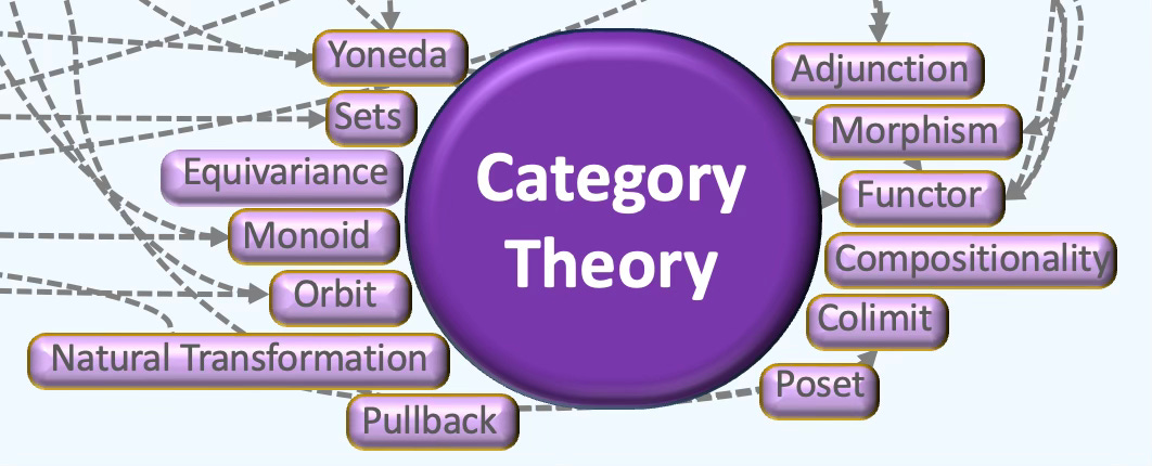
🪢 Category Theory
Category theory offers a panoramic view of mathematics: it suppresses detail to reveal structure. From this vantage, unexpected parallels emerge—why the least common multiple mirrors a direct sum, or what discrete spaces, free groups, and fraction fields share.
Applicability
Category theory can be used to generate composable guarantees (equivariance, conservation, privacy), building large, reusable ML systems for which algebraic laws are refactored.
Compositional modeling such as functors, morphism and natural transformations for clean modularity, correctness-by-construction, and reusable connecting laws for complex systems
Monoidal categories to reason about neural architectures and algebraic dataflow such as fork/join,or skip connections) and validate equivalences
Categorical automatic differentiation which defined back-propagation as a functor and derivative as algebraic operator (lenses)
Probabilistic reasoning using Markov categories, monads for compositional probabilistic programming semantics and modular inference with glue samplers & posteriors)
Equivariance & symmetries for which group actions as defined as functor to design equivariant neural layers (translations/rotations/permutes) with invariances/equivariance
Graphs & sheaves to enforce multi-scale constraints, and principled higher-order architectures as applied in topological deep learning (simplicial neural networks).
Operads for safe composition of reusable blocks, specifying how smaller models plug into larger ones or compose along interfaces
Kernels & categorical approximation to explain polynomial/spectral graph filters and universal kernels.
Key Concepts
Objects & Morphisms
A category is a system of related mathematical objects with maps that bind them together. Example of an object is a group or topological space while a map can be a morphism [ref 39]. Interestingly enough, a category is also an object. Set, Group, Ring and Toph are the most common categories. Category theory is intimately linked to algebraic topology described in a previous section [ref 40]. Categories without maps are known as discrete categories.
Set is a category whose objects are small sets, morphism ordinary functions, identity is the identity function and composition is the composition of functions.
Ring is an algebraic structure and a category: a set equipped with two binary operations—addition and multiplication—that satisfy the familiar laws of integer arithmetic, Rings are usually not commutative. The category of integers is a ring.
Top is a category of topological spaces equipped with a basepoint, together with the continuous basepoint-preserving maps
A subcategory of a category consists of a subclass of object contained in the category.
Besides containing objects and associated maps/morphisms. categories support associativity, composition and identity laws.
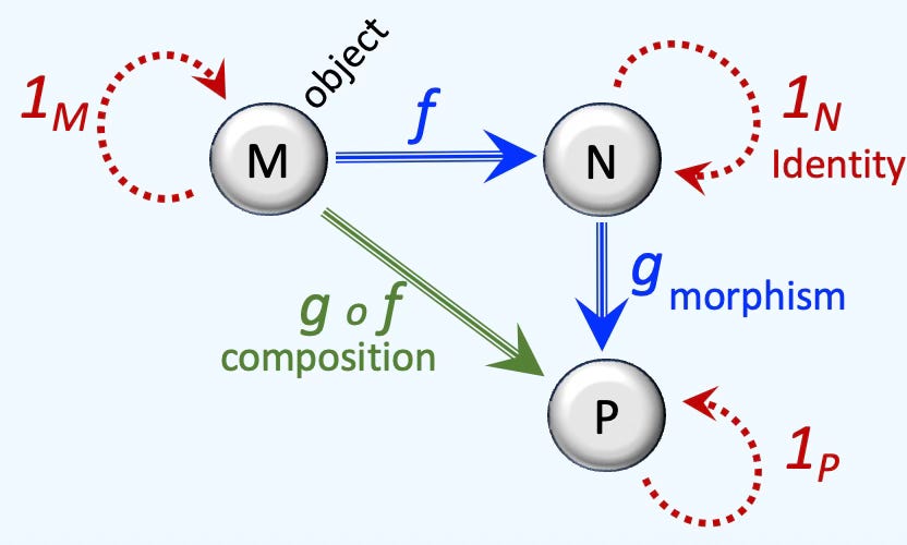
A monoid is a set category equipped with an associative binary operations and two-sided unit element. A preorder is a reflexive transitive binary relation.
The principle of duality, fundamental to category theory. states that every categorical definition, theorem and proof has a dual, obtained by reversing all the maps.
Functors
A functor is a morphism between categories for which, for any object
The functor of the composition of two maps is the composition of the functors of each of the maps
The functor of identity if the identity of the functor.
Functors arise in algebraic topology: they associate the categories of topological spaces to the category of algebras such as Lie algebra or Abelian algebras [ref 39]. A functor is faithful is function over two objects is injective.
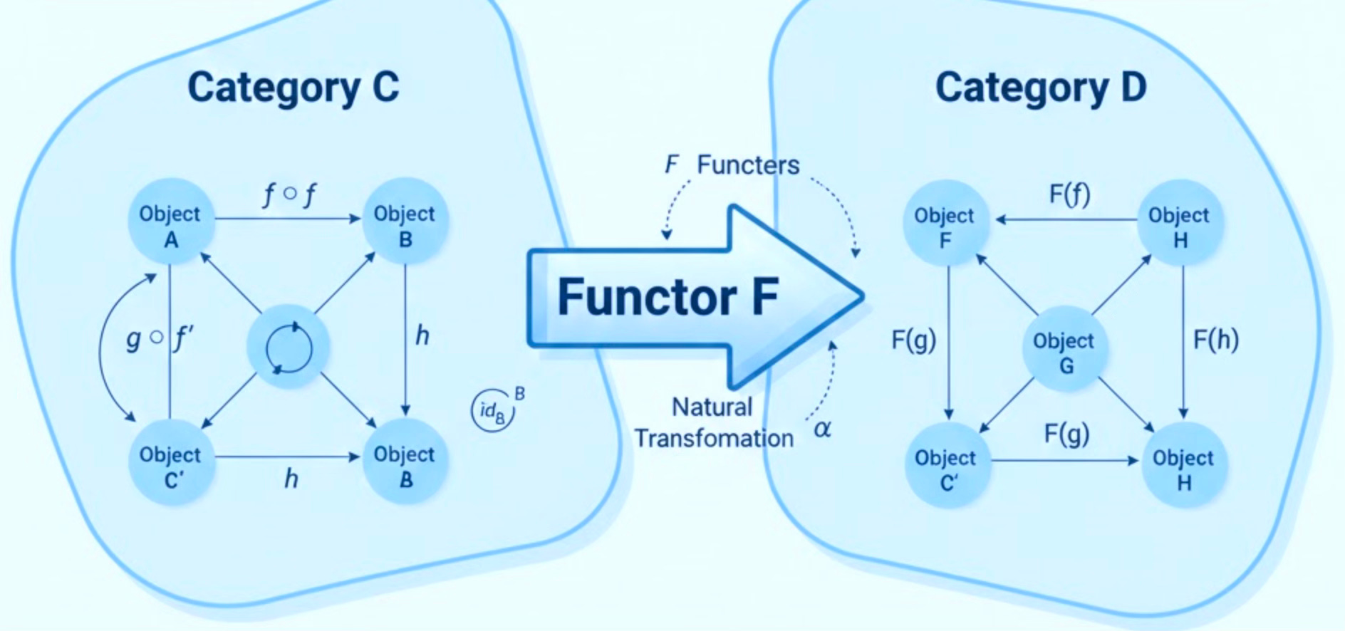
A contravariant functor associates any object from M to an object of N such F(gof) = F(f) o F(g). For a covariant (or ordinary) functor, F(gof) = F(g) o F(f). A contra variant functor is a covariant functor on the opposite category.
An adjunction is a relationship between two functors that captures a weak form of equivalence between their categories. Functors in this relationship are called adjoint—one is the left adjoint, the other is the right adjoint [ref 41]. Such pairs are ubiquitous and often arise from “best” or optimal constructions.
Natural transformations are morphisms between functors which assign morphism to each object of a given category.
The Yoneda lemma is fundamental in category theory. It states that knowing how every other object maps into or out of an object is enough to ‘know’ this object.
Sheaves & Topos
Sheaf theory sits at the crossroads of geometry, algebra, and category theory. It associates to each part of a geometric space data drawn from a target category (e.g., sets, vector spaces), embedding the space into a richer computational setting for representation and processing [ref 42].
A sheaf assigns data (e.g., sets, rings) to the open sets of a topological space, with rules ensuring locality and consistent gluing. Maps between sheaves (morphisms) are defined in the usual way. Sheaves play a central role in algebraic and differential geometry. A topos is a category modeled on sheaves of sets over a space. Like Set, topoi have set-like structure and support localization. Grothendieck topoi are central in algebraic geometry, while elementary topoi are widely used in logic.
Generator-Filter Theory
This theory relies on a pair Generator-Filter. A generator is an object that can ‘generate’ the entire category, meaning that any object or structure in the category can be constructed or represented from the generator. A filter is a concept of selection and constraint within a system, often used in the context of ‘filtered categories’.
Abridged Glossary - 5
2-cell: A transformation between 1‑cells.
Adjunction: A pair of functors L ⊣ R with unit and counit laws.
Bicategory: Generalization of categories with objects, 1‑cells, and 2‑cells.
Category: A collection of objects and morphisms (arrows) between them with associative composition and identity arrows.
Co-limit: The most general way to generate and weave a diagram in a category such as a disjoint union in a set.
Co-monad: Dual monad with a corresponding co unit and co multiplication.
Equivariance: Property of applying the symmetry then an action is equivalent to applying an action then a symmetry
Fibration: A functor satisfying certain lifting properties, often modeling families of structures indexed by base objects.
Functor: A structure-preserving map between categories.’
Groupoid: Category where every morphism is invertible.
Monad: A functor with unit (η) and bind (≫=) satisfying laws; captures effects.
Monoid: A set with an associative binary operation and identity element.
Monoidal structure: Category with a tensor product and unit object.
Morphism (Arrow): A relation or transformation between objects.
Natural transformation: A systematic way of converting one functor to another while commuting with morphisms.
Poset: Category with at most one arrow between objects.
Pullback: Universal construction combining two morphisms with a common codomain (a.k.a. Fiber product).
Pushout: Dual to pullback, universal merging along a shared part.
Object: An entity in a category.
Orbit: An equivalence class generated by the action on an object of a given category
Sub-object classifier: An arrow indicating membership.
📘 References
Geometric deep learning: going beyond Euclidean data M. Bronstein, J. Bruna, Y. LeCun, A. Szlam and P. Vandergheynst - 2017
Geometric foundations of Deep Learning - M. Bronstein - 2025
Geometric Deep Learning Book M. Bronstein, J. Bruna, T. Cohen, P. Veličković
Introduction to Geometric Deep Learning - Hands-on Geometric Deep Learning, 2025
Mathematical Foundations of Geometric Deep Learning H. S. de Ocariz Borde, M. Bronstein - University of Oxford, 2015
Introduction to Smooth Manifolds J. Lee - Springer Science+Business media New York 2013
Riemannian Manifolds: Foundational Concepts - Hands-on Geometric Deep Learning, 2025
Differential Geometry - Tensor Calculus - R. Davie - YouTube, 2024
Differential Geometry - Khan Academy - YouTube, 2024
Tensor Analysis on Manifolds - Chap 1: Manifolds R Bishop, S. Goldberg - Dover Publications, New York 1980
Differential Geometric Structures- Chap 3: Riemannian Vector Bundles W. Poor - Dover Publications, New York 1981
Tensor Analysis on Manifolds - Chap 5: Riemannian Manifolds R Bishop, S. Goldberg - Dover Publications, New York 1980
Tensor Analysis on Manifolds - Chap 3: Vector Analysis on Manifolds R Bishop, S. Goldberg - Dover Publications, New York 1980
Algebra, Topology, Differential Calculus, and Optimization Theory For Computer Science and Machine Learning J. Gallier, J. Quaintance - Dept of Computer and Information Science - University of Pennsylvanian, 2025
SE(3): The Lie Group That Moves the World - Hands-on Geometric Deep Learning, 2025
Mastering Special Orthogonal Groups With Practice - Hands-on Geometric Deep Learning, 2025
Introduction to Lie Groups and Lie algebras Chap 1 & 2 - A Kirillov. Jr - SUNNY at Stony Brook
Differential Geometric Structures- Chap 7: Symmetric Spaces W. Poor - Dover Publications, New York 1981
Differential Geometric Structures- Chap 8: Symplectic and Hermitian Vector Bundle W. Poor - Dover Publications, New York 1981
Algebraic Topology for Data Scientists M. Postol - The MITRE Corporation, 2024
Topology - Chap 2: Elements of Point-Set Topology J. Hocking, G. Young - Dover Publications, 1988
Topology - Chap 4: The Elements of Homotopy Theory J. Hocking, G. Young - Dover Publications, 1988
From Nodes to Complexes: A Guide to Topological Deep Learning - Hands-on Geometric Deep Learning, 2025
Exploring Simplicial Complexes for Deep Learning: Concepts to Code - Hands-on Geometric Deep Learning, 2025
Topology - Chapter 6: Simplicial Homology Theory J. Hocking, G. Young - Dover Publications, 1988
Chain Complexes - MIT Libraries, 2021
Introduction to Differential Geometry Chap 6 De Rham Cohomology J. Robbin,
D. Salamon UW Madison, ETH Zurich, 2025
Sheaf Theory Perspectives: Insights and Applications G. Magal - Medium, 2025
Graph Theory Schaum’s Outlines - V. K. Balakrishnan, 1997
Introduction to Graph Theory Chap 1 Definition and Examples R. Wilson - 4th Edition - Addison-Wesley 1996
An introduction to Graph Theory - Chap 3 Multigraphs D. Grinberg - Drexel University, Korman Center - 2025
Spectral Graph Theory D. Spielman - Yale University, 2011
A Short Tutorial on the Weisfeiler-Lehman Test and its Variants N. Huang, S. Villar - Applied Mathematics and Statistics, John Hopkins University, 2022
Graph and Matrices - R. B. Bapat - Springer, 2009
The Many Faces of Information Geometry F. Nielsen - Notices of the American Mathematical Society, 2022
An Elementary Introduction to Information Geometry F. Nielsen - Sony Computer, 2 Science Laboratories, 2020
What is Fisher Information? Ian Collings - YouTube, 2024
Shape your Model with Fisher-Rao Metric - Hands-on Geometric Deep Learning, 2025
Basic Category Theory - Chap 1: Categories, Functors and Natural Transformations - T. Leinster - University of Edinburgh, 2025
Category Theory in Machine Learning D. Shiebler, B. Gavranovic’, P. Wilson - University of Oxford, Strathclyde, Southampton, 2021
Basic Category Theory - Chap 2: Adjoints - T. Leinster - University of Edinburgh, 2025
Sheaf Theory Perspectives: Insights and Applications G. Magai - Medium, 2025
Curvature-informed Graph Learning - Hands-on Geometric Deep Learning, 2026
Reader classification rating
⭐ Beginner: Getting started - no knowledge of the topic
⭐⭐ Novice: Foundational concepts - basic familiarity with the topic
⭐⭐⭐ Intermediate: Hands-on understanding - Prior exposure, ready to dive into core methods
⭐⭐⭐⭐ Advanced: Applied expertise - Research oriented, theoretical and deep application
⭐⭐⭐⭐⭐ Expert: Research , thought-leader level - formal proofs and cutting-edge methods.
Share the next topic you’d like me to tackle.
Patrick Nicolas is a software and data engineering veteran with 30 years of experience in architecture, machine learning, and a focus on geometric learning. He writes and consults on Geometric Deep Learning, drawing on prior roles in both hands-on development and technical leadership. He is the author of Scala for Machine Learning (Packt, ISBN 978-1-78712-238-3) and the newsletter Geometric Learning in Python on LinkedIn.
Never in my life I thought that such things as topology and deep learning geometry will be a practical tool to use in my professional life. But here I am explaining to myself and my colleagues the inner workings of llm with such fancy terms. Thnx for the article- great stuff!