

Visualization Tools for Geometric Deep Learning
Expertise level: ⭐

Have you ever found it challenging to translate complex AI architectures or machine learning outcomes into a clear, compelling narrative?
Fortunately, Python offers a powerful suite of libraries specifically designed to bring these models and concepts to life through visualization and animation.


🎯 Why this Matters
Purpose: Abstract mathematical frameworks, including algebraic topology and differential geometry, are often best elucidated through dynamic visualizations and animations. These tools are invaluable for both conceptual demonstrations and the interpretation of experimental results. To meet this need, the Python ecosystem offers data scientists a robust selection of specialized animation libraries.
Audience: Scientists and engineers who needs to describe their model through animation or create demos to illustrate a new concept
Value: Explore essential Python libraries as powerful communication vehicles for visualizing and animating complex models and experimental results.
🎬 Animation Frameworks
📌 Although various specialized 3D rendering frameworks are available [ref 1], they are often either underutilized in research or incompatible with the requirements of geometric learning.
Matplotlib/Animation
While Matplotlib remains the industry standard for static and interactive data visualization, its animation features are frequently underutilized and less widely understood.
📌 This article focuses specifically on animation; therefore, I will not delve into Matplotlib’s standard plotting functionality.
Functionality
While often seen as “basic,” Matplotlib remains the most versatile for scientific plotting and is often the best “first step” for simple animations. It is best suited for Real-time signal processing, simple 2D dynamic systems, physics and math simulation [ref 2].
Matplotlib enables animation generation via its animation module, treating an animation as a series of individual frames plotted on a single, condensed figure.
The animation process relies on two Python classes [ref 3].
FuncAnimation that generates animation by iteratively updating the data of a single plot. It is generally the more efficient choice for memory and speed.
ArtistAnimation that creates animation from a pre-defined list of “Artist” objects (drawings) for each frame. This approach is better suited for complex or highly creative scenes.
Installation
pip install matplotlibBasic design is illustrated by the following pseudo-code
draw:
   initialize animation configuration parameters
   set up static elements
   -> update(frame)   # Nested function to update the dynamic component

   invoke FuncAnimation(fig, update, frames=100, interval=300, ...)
   save animation to MP4 file
Manim
Manim is the gold standard for high-quality, explanatory math videos. It is particularly suitable for Calculus, linear algebra, and complex equations where precise “morphing” between formulas and shapes is needed. Manim is the most commonly used animation on YouTube [ref 4].
The key features are Native LaTeX support, built-in coordinate systems, and beautiful object to object transformations.
Functionality
A Manim animation implements a dynamic scene, defined in the class Scene (or its subclasses). Objects to be displayed and/or animated in a scene have their type inheriting from the class Mobject [ref 5, 6]
Here a list of the most common objects, scenes and animation functions.
Objects
Mobject: base class for objects that can be displayed on screen.
VMobject: A vectorized Mobject
VGroup A group of vectorized objects of type VMobject
NxGraph: Generic mathematical graph
Graph: Undirected graph
DiGraph: Directed graph
ValueTracker: An object that track real-value parameters
Arc: A circular arc defined by its start and end angle (radiants)
Circle: A circular arc (0, 2.pi)
Line: A curved or straight line between 2 mobjects
Arrow: Graph configuration arrow
Text: Ascii or Latex content
Angle: A circular arc mobject defined by its angle
…
Scenes
Scene: Set of tools to manage mobject and animations
ThreeDScene: 3D scene with camera angle
SpecialThreeDScene: 3D scene with support for spheres and camera shades
The key functions for scenes are
construct: Add content mobjects or vmobjects to the scene
add: Adds a mobject
clear: Removes all objects
remove: Removes a given mobject
bring_to_front/bring_to_back: Brings mobjects in front or back in the scene
pause : Pauses the scene
play: Plays an animation in the scene
wait: Plays animation without change
Animation
Create: Shows a mobject
Write: Simulate hand-drawing or handwriting
Unwrite: Simulate the erasure of handwriting or hand-drawing mobject
FadeIn: Alternative to create by fading in an mobject into the scene
FadeOut: Fades out an mobject into the scene
Rotate: Animation that rotates an mobject in a scene
Transform: Transform one mobject to another one
…
📌 ManimGL is a separate version of Manim (by 3Blue1Brown) that uses OpenGL for hardware-accelerated, real-time rendering. If you find the standard ManimCE too slow for your complex manifolds, ManimGL might be the solution.
Installation
Installation Linux
sudo apt update
sudo apt install build-essential python3-dev libcairo2-dev
                 libpango1.0-dev ffmpeg   # Manim dependency
pip install manim
Installation MacOS
brew install manim
brew install py3cairo ffmpeg pango pkg-config scipy     # Dependencies
Installation verification
manim checkhealthInitializing a Manim project in folder ‘my_folder’
manim init project my-folder --defaultExecution of a scene - class MyScene
manim -pql main.py MyScene
ql: low quality video
qm: medium quality video
qh: high quality video
📌 Although the Seaborn library is a compelling extension to Matplotlib plotting capabilities, it does not support animation.
Which Animation Library?
Choosing between Matplotlib and Manim depends entirely on whether you are analyzing data or explaining a story. Matplotlib is built for speed and scientific rigor, while Manim is built for cinematic, educational aesthetics.

📌 Beyond Matplotlib and Manim, two additional frameworks provide the sophisticated 3D rendering capabilities required for complex tasks:
PyVista, which excels at generating 3D manifolds and intricate surface meshes [ref 7].
Plotly, which is optimized for developing interactive dashboards for real-time analysis and monitoring [ref 8]
⚙️ Hands‑on with Python
Environment
Libraries: Python 3.12.5, Numpy 2.3.5, Pandas 3.0.0, Matplotlib 3.10.1, Seaborn 0.13.2, Manim 0.19.2
Evaluation code (Github):
animation/manim_neighbor_loader.py
The source tree is organized as follows: features in python/, unit tests in tests/,and newsletter evaluation code in play/.
To enhance the readability of the algorithm implementations, we have omitted non-essential code elements like error checking, comments, exceptions, validation of class and method arguments, scoping qualifiers, and import statements.
Use Cases
Lie SE3 Euclidean Group (Matplotlib Animation)
The SE3 Lie group is fully described in a previous article [ref 9] . As a quick reminder, the SE3 Lie group transformation is defined as: SE(3): The Lie Group That Moves the World
This implementation uses FuncAnimation frame-based simulator with the update (stepping) method implemented as a nested function.
🔎 Implementation
Let’s wrap the animation of SE3 manifold (Rotation + Translation) into a class, SE3Animation.
The constructor has two arguments:
transform That implement the 4x4 SE(3) transformation matrix on the smooth manifold
kwargs: Optional extra configuration parameters
The constructor initializes the static elements of the simulation (fig, ax, ) and initial the parameterized trajectory next_step

The actual animation if implemented by the method draw in code snippet 2. First, we setup the trajectory of the sphere to illustrate the translation component of the SE(3) transformation. The geodesic lines, created in the method __sphere_geo_lines that visualizes the rotation of the sphere are initialized along the initial location of the sphere (__draw_trajectory) and the sphere in 3D space (__draw_sphere).

The code snippet illustrates how to leverage the function FuncAnimation and ffmpeg library to generate a MP4 file.
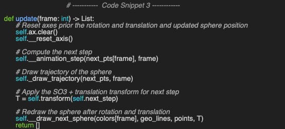
The method update adjusts the dynamic components of the animation at each new frame is implemented in the code snippet 3.
The list components to be updated at each frame are
New location of the sphere next_pts (Translation)
Sphere rotated by the transformation T and display by the method __draw_next_sphere
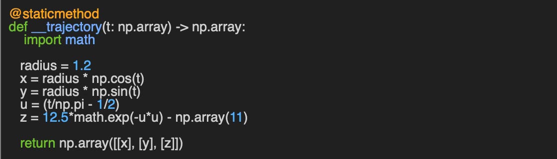
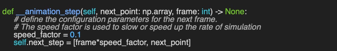
Two worth noting methods - __trajectory that specify the trajectory of the sphere in 3D ambient Euclidean space and __animation_step that specifies the rate of simulation per frame - are described in Appendix
⚠️ For performance purpose it is highly recommended to exclude any static visual components such as formulas, title, legend… from the method update.
Animation
The execution of the animation is very simple as it only requires defining the transformation (SE3) default_se3_transform and the visual configuration parameters config.

The resulting MP4 can be executed directly through the browser
Video 1: Visualization of the SE(3) transformation of a sphere using Matplotlib/Animation
Graph Convolutional Neural Network (Manim)
A Graph Neural Network (GNN) is an optimizable transformation on all attributes of the graph (nodes, edges, global context) that preserves graph symmetries (permutation invariances). GNN takes a graph as input and generate/predict a graph as output [ref 10]
Data on manifolds can often be represented as a graph, where the manifold’s local structure is approximated by connections between nearby points. GNNs and their variants (like Graph Convolutional Networks (GCNs) extend neural networks to process data on non-Euclidean domains by leveraging the graph structure, which may approximate the underlying manifold.
📌 While Manim supports more complex features, this animation was chosen because it highlights the engine's core functionality, including groups, object linking, LaTeX integration, and camera angle rotation
🔎 Implementation
Let’s define our animation as a 3D scene and therefore create a subclass of Manim ThreeDScene - ManimNeighborLoader.
We override the method Manim construct to
Load and initialize the graph with a single central node and its immediate neighbors - hop_1
Create a Vgroup to visualize the nodes around a first node, center_dot
Initialize and create the neighboring nodes with their labels
Fade in/display the central node
Fade in its neighbors in hop_1 set

Create the graph edges- edge_objs
Update the labels and the latex formula matmul
Visualize the message massing and aggregation using Manim Arrows mobjects
Display the formula for the message aggregation - sum_symbol

Display the rotation of the sphere as illustrated by the redrawing of the geodesic lines
Display the Latex formula for the activation function
Modify the color of the central node
Display the latex formula to update the node’ features

Animation
Once the MP4 file is generated, the video is run through the command line
manim -pql main.py ManimNeighborLoader
Video 2: Visualization of message passing and aggregation in a graph convolutional network using Manim
📌 Since Manim can take a while to render high-res MP4s, the best approach is ‘render low, release high.’ Use manim -pql while you’re building the animation to see changes instantly, then bump it up to -qh for your finished product.
🧠 Key Takeaways 💎
✅ Matplotlib.animation: An accessible extension of the standard Matplotlib library, offering a gentle learning curve for those looking to add dynamic updates to existing visualizations.
✅ Manim: A high-fidelity engine supporting complex scenes, camera controls, and LaTeX integration; however, its extensive feature set requires a significantly higher time investment to master.
✅ Use Cases: Matplotlib excels in real-time monitoring and data analysis, whereas Manim is optimized for polished educational content, professional demonstrations, and high-quality storytelling.
✅ Performance: Due to its rendering overhead, Manim is less efficient for large-scale sequences. It is best used with a “low-quality first” iterative workflow, scaling up to high-resolution output only for the final release.
📘 References
Python Libraries for Mesh, Point Cloud, and Data Visualization
Manim Tutorials - manim.org
Manim Community - manim.org
Manim Example Scenes - manim.org
SE(3): The Lie Group That Moves the World - Hands-on Geometric Deep Learning, 2025
Graph Convolutional or SAGE Networks? - Hands-on Geometric Deep Learning, 2025
🛠️ Q & A 💎
Q1: What is the primary performance limitation when utilizing Manim for large-scale model animations?
Q2: Which of the most common Matplotlib API functions is responsible for managing animations on a frame-by-frame basis?
Q3: What is the standard method used to define and construct a Scene within the Manim framework?
Q4: Which animation library provides native, comprehensive support for dynamic LaTeX rendering?
Q5: What is the correct CLI command to render a specific scene - NewScene - in Manim medium quality video?
👉 Answers
🧩 Appendix 💎
Animation of Lie groups with MatplotLib
Sphere Trajectory
The trajectory is defined by the simple f(x(t), y(t), z(t)) for illustration purpose (t = frame)
The following code snippet is a direct implementation of the formula above. The parameters alpha and beta is used to keep the sphere within the boundary of the plot.
Animation step for Sphere
💬 News & Reviews 💎
This section focuses on news and reviews of papers pertaining to geometric deep learning and its related disciplines.
Paper Review: GGNNs : Generalizing GNNs using Residual Connections and Weighted Message Passing A. Raghuvanshi, Kushal S M - Dept. of Aerospace Engineering - Indian Institute of Technology, Bombay, 2023
Graph Neural Networks (GNNs) and their message-passing or aggregation mechanisms are well suited to capturing structural relationships and patterns in graph datasets, enabling accurate node classification and prediction.
The authors propose a Generalized Graph Neural Network (GGNN) that extends traditional GNNs with two key enhancements:
Residual connections, inspired by architectures such as CNNs and ResNets.
Learnable message weights, which adapt based on the relevance of information carried by each edge.
1. Residual connections
Each hidden layer’s output is combined with the affine-transformed output of the preceding neural layer (MLP) through a scaled residual connection. This design improves information flow without increasing computational complexity. To ensure dimensional consistency, the previous layer’s output length is adjusted via a max-pooling operation.
2. Learnable weights
Each edge in the graph is assigned a trainable weight computed from the degrees of its two incident nodes. These weights encode the relative importance of messages, allowing the model to emphasize more informative connections during aggregation.
Evaluation
The GGNN is evaluated against a baseline message-passing GNN and a Perceptual Message-Passing MLP using benchmark datasets from PyTorch Geometric (Cora and Citeseer). The proposed model achieves performance improvements of 4% to 26% on test sets while requiring only half the number of training epochs compared to the baselines.
Note: Performance improvement could be more significant for inductive Graph Neural Network such as GraphSAGE
Share the next topic you’d like me to tackle.
Patrick Nicolas is a software and data engineering veteran with 30 years of experience in architecture, machine learning, and a focus on geometric learning. He writes and consults on Geometric Deep Learning, drawing on prior roles in both hands-on development and technical leadership. He is the author of Scala for Machine Learning(Packt, ISBN 978-1-78712-238-3) and the newsletter Geometric Learning in Python on LinkedIn.