Understanding Data Through Persistence Diagrams

Expert level: ⭐⭐⭐

Persistence diagrams are cornerstones of Topological Data Analysis, yet the formal algebraic topology required to understand its foundations can be intimidating for readers without a strong mathematical background. This article aims to bridge that gap.

1. 🎯 Why this Matters

2. 🎨 Modeling & Design Principles

   Overview

   Topological Data Analysis

   Persistent Homology

   Persistence (Birth-Death) Diagram

   Persistence Image

   Persistence Landscape

3. 📚 Python Libraries

   Scikit-learn TDA

   Ripser

   Persim

4. ⚙️ Hands-on with Python

   Environment

   Shaped data sets

   Persistence Diagrams

5. 🧠 Key Takeaways 💎

6. 📘 References

7. 🛠️ Exercises 💎

8. 🧩 Appendix 💎

9. 💬 News & Reviews 💎

🎯 Why this matters

Purpose: I have already introduced simplicial complexes, cell complexes, and hypergraphs as core tools in Topological Data Analysis. It is now time to turn to persistent homology, beginning with persistence diagrams as a way to capture global geometric structure and extract topological features.

Audience: Data scientists and machine learning engineers aiming to assess the underlying shape and structure of data prior to building models.

Value: Learn to recognize and interpret the most common persistence diagrams using noisy, shape-driven data.

🎨 Modeling & Design Principles

Overview

I already dived into the key components of topological data analysis - topological spaces, and domains such as simplicial complexes or cell complexes - as a pre-requisite to the introduction of homology [ref 1].

---

📌 The topological concepts such as topological spaces, complexes or filtration and related terminology is described in Demystifying the Math of Geometric Deep Learning - Topology

---

This article considers only topological spaces equipped with.a metric with emphasis on simplicial complexes described in a previous article - Exploring Simplicial Complexes for Deep Learning: Concepts to Code

Topological data Analysis

---

⚠️ I emphasize that this paper is not a survey of recent advances in topological data analysis, but rather a tutorial designed to introduce the basic concepts to machine learning practitioners

---

Many challenges in data analysis echo two fundamental integration problems:
how to recover high-dimensional structure from low-dimensional representations, and how to assemble discrete samples into a coherent global form.

Persistent Homology enhances unsupervised learning by redirecting attention from local structures to global topological invariants—features that remain stable under continuous deformations. It does so by building a sequence of nested simplicial complexes, known as a filtration.

Persistent Homology offers a great feature extraction method for complex datasets, not always possible by traditional unsupervised methods.

As a quick reminder, In the simplest terms, a simplicial complex is a graph with faces. It generalizes graphs that model higher-order relationships among data elements—not just pairwise (edges), but also triplets, quadruplets, and beyond (0-simplex: node, 1-simplex: edge, 2-simplex: Triangle, 3-simplex: Tetrahedron, ) [ref 2].

Persistent Homology

Homology is a mathematical operation whose inputs are topological spaces and outputs are groups.

Persistent homology offers a means to capture the global geometric and topological structure of complex data by identifying and tracking features such as loops, cycles, and voids across multiple scales [ref 5, 6].

Persistent homology can be summarized as a three-step procedure as follows:

1. Filtration: Generate a nested sequence of simplicial complexes derived from the data. Through filtration, Persistent Homology tracks the emergence and disappearance of topological features across multiple scales, revealing structural properties of the data that traditional methods often miss.

2. Persistence diagrams: Record the evolution of topological features across this sequence.

3. Machine learning integration: Transform the persistence diagrams into vectors for efficient use in ML models [ref 1].

This article focuses on persistence diagrams.

---

📌 Persistent barcodes are algebraic invariant alternative to persistent diagrams. They are beyond the scope of this article and the subject of a future article on persistent homology [ref 7]

---

Persistence (birth-death) Diagram

A persistence diagram maps the “birth” (appearance) and “death” (disappearance) times/scales of topological features such as cavities, holes or connected components in a dataset as a collection of points in a 2D plot. It represents the “fingerprint” of the data’s shape, with points far from the diagonal indicating significant features and those near the diagonal suggesting noise.

Fig. 1 Features vs Noise on a 2D Persistence Diagram

A filtration is defined as a sequence of topological Xi spaces of increasing size

\(F =X_{0} \subseteq X_{1} \subseteq \ ... \ \subseteq X_{n}\)

The dimension of the homology group is defined as

• k=0: Connected components

• k=1: Loops

• k=2: Cavities

• …

The k-th homology groups Hk for each of the topological space Xi and its induced linear map i associated to the inclusion:

\(\left\{ H_{k}(X_{0}), H_{k}(X_{1}), \ .... \ ,H_{k}(X_{h}) \right\} \ \ \ \ i_{p\to q}: \ H_{k}(X_{p})\to H_{k}(X_{q}) \ \ \ p \le q \)

The homology class [C] of k-th homology of topological space Xi, Hk(Xp) is born at index p =b and dies at index q = d (= inf if no death)

\(i_{b \to d}([C]) = 0\)

Given each persistence interval [bj, dj], the persistence diagram dgm[k] for nth homology class is then defined as

\(dgm_{k}(X)=\left\{ (b_{j}, d_{j}) \ | \ i_{b_{j} \to d_{j} } ([C])=0 \right\}\)

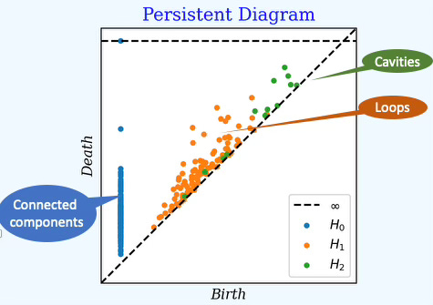
Fig. 2 Persistence Diagram for a Torus-shaped 256 data points with 15% noise

Interpretation:

• x-axis (Birth): filtration value where a feature appears

• y-axis (Death): filtration value where it disappears

• Diagonal y=x zero persistence (pure noise)

• Distance to diagonal: feature importance

Colors / legend:

• 🔵 Blue → H0 (connected components)

• 🟠 Orange → H1 (loops / cycles)

• 🟢 Green → H2 (voids / cavities)

• ∞ bar (dashed horizontal) → never-dying component

Persistence Images

Persistence images transform persistence diagrams into gridded numerical images that can used as feature vectors to classical machine learning algorithms (SVM, Random forest,) or deep learning architectures. Bright colors represent high persistence while fainted colors represents low persistence. Persistence images preserve essential topological structure while giving a stable, computable representation.

---

📌 Persistence images are referred as topological fingerprint or topological heatmap.

---

The construction of a persistence image involves three steps:

1. Express each feature in birth (b)–persistence (d) coordinates, with x=b and y=p=d−b

2. Smooth every point (b, p) using a Gaussian kernel.

   \(\begin{matrix} \rho_{b, p}(x, y) = w_{b, p}.exp\left( -\frac{(x-b)^2)+(y - p)^2}{2\sigma^2} \right) \ \ \\ \sigma: \ smoothing \ parameters \ \ \ \ \ \ \ \ \ \ \ \ \ \ \ \ \ \ \ \\ w_{b,p}: \ weight \ of \ the \ persistence \ \ \ \ \ \ \ \ \ \ \ \end{matrix}\)

3. Sample the resulting birth–persistence density over a 2D grid of cells [k,ℓ]

\(pi_{k,l}=\int_{}^{}\int_{[k,l]}^{} \sum_{j\in [k,l]}^{}\rho_{j}(x, y)dxdy\)

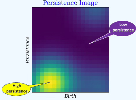
Fig. 3 Persistence image from a Swiss Roll-shaped 384 data points with 20% noise

Interpretation:

• x-axis (Birth): filtration value where a feature appears

• y-axis (Persistence = Death − Birth): lifetime of that feature

• Color intensity: weighted density of features (usually Gaussian kernels weighted by persistence). Bright regions correspond to clusters of persistent homological features.

---

📌 Persistence images are used for periodicity detection in time series, biological data and Physics-informed deep learning.

---

Persistence Landscapes

Persistence landscapes turn persistence diagrams into functions in a Hilbert space that preserve topological information. It is essentially a summary of how many features are alive at each scale and how strong they are. Usually the tail values highly the important topological features.

Given a pair of births, b and deaths d in a persistence diagram we generate the following triangular function known as landscape layers:

\(\lambda(t)= \begin{Bmatrix} t-b & if \ t \in \left[b,\frac{b+d}{2} \right] \\ d - t & if \ t \in \left[\frac{b+d}{2}, d \right] \\ 0 & otherwise \ \ \ \ \ \ \ \ \end{Bmatrix}\)

The lambdas are ordered in decreasing order of values.

\(\Lambda_{n}=\left\{ \lambda_{0}(t) \leqslant \lambda_{1}(t) \leqslant \ ... \ \leqslant \lambda_{n}(t)\right\}\)

The commonly listed benefits are

• Support for statistical computation such as average, norm and hypothesis testing

• Preservation of magnitude of changes reflected in the landscape (data → triangle)

• Conversion of topological feature into either function (Hilbert space) or vectors, suitable for traditional machine learning algorithm such as deep learning or support vector machines.

The computation of the landscape layers or functions is costly for large digram. An approximation, approximate landscape, discretizes these functions through sampling over a finite grid. This is the most commonly used version of the persistence landscape.

The strict, mathematical implementation of the landscape functions, known as exact landscape relies on the piecewise linear representation.

---

📌 There are few more diagrams such as Persistent Laplacian Diagrams which extend persistent homology by using the combinatorial Laplacian—rather than boundary maps—to study how geometric and topological structures evolve across a filtration.

---

Interpretation:

A persistence landscape is a functional summary of a persistence diagram:

• x-axis: filtration parameter

• y-axis: landscape value (height of the k-th most persistent feature at that scale)

• λ1 captures the strongest feature,
  λ2 the second strongest,

  …

At any filtration value t, the landscape stacks the top-k surviving features.

📚 Python Libraries

Scikit-TDA

The scikit-learn TDA package generally refers to the ecosystem of Topological Data Analysis tools that follow the scikit-learn API, most notably the packages from the scikit-tda organization [ref 8].

Practically, scikit-tda is a collection of Python libraries that bring Topological Data Analysis techniques into the scikit-learn workflow such as:

• Persistent homology & persistence diagrams

• Vietoris–Rips complexes

• Topological feature vectors

• Machine-learning models leveraging topological domains

Scikit-learn TDA leverages two 3rd party packages

• Ripser for fast persistent homology computation

• Persim for creating and visualizing persistence diagrams

Installation:

pip install scikit-tda

Ripser

Ripser.py is a lean persistent homology package for Python built upon the fast C++ Ripser engine [ref 9]. It supports:

• Computing persistence homology & cohomology

• Handling both sparse and dense data sets

• Approximating sparse filtration

• Visualizing persistence diagrams

• Computing lowerstar filtrations on images

• Computing representative cochains.

Installation:

pip install Cython
pip install Ripser

Persim

Persim is a Python package for analyzing Persistence Diagrams. Its functionality covers key methods used in TDA:

• Persistence images and landscape

• Distances such as bottleneck

• Kernels such as Heat and Wasserstein

• Out-of-the-box plotting capabilities

⚙️ Hands‑on with Python

Environment

• Libraries: Python 3.12.5, Numpy 2.3.5, scikit-learn 1.7.0, Scikit-TDA1.1.1, ripser 0.6.12, persim 0.3.8

• Implementation: geometriclearning/topology/homology/persistence_diagrams.py

  Evaluation: geometriclearning/topology/homology/persistence_diagrams_play.py

• The source tree is organized as follows: features in python/, unit tests in tests/,and newsletter evaluation code in play/.

• To enhance the readability of the algorithm implementations, we have omitted non-essential code elements like error checking, comments, exceptions, validation of class and method arguments, scoping qualifiers, and import statements.

Shaped-data set

The visualization of persistence diagrams is illustrated using pre-defined shape (or manifold) for the data with added noise.

The following three 3D plots illustrate the noisy data embedded in a manifold. The red dot represents data points defined as data_from_shape*(1 + 0.2*noise[0, 1])

Sphere

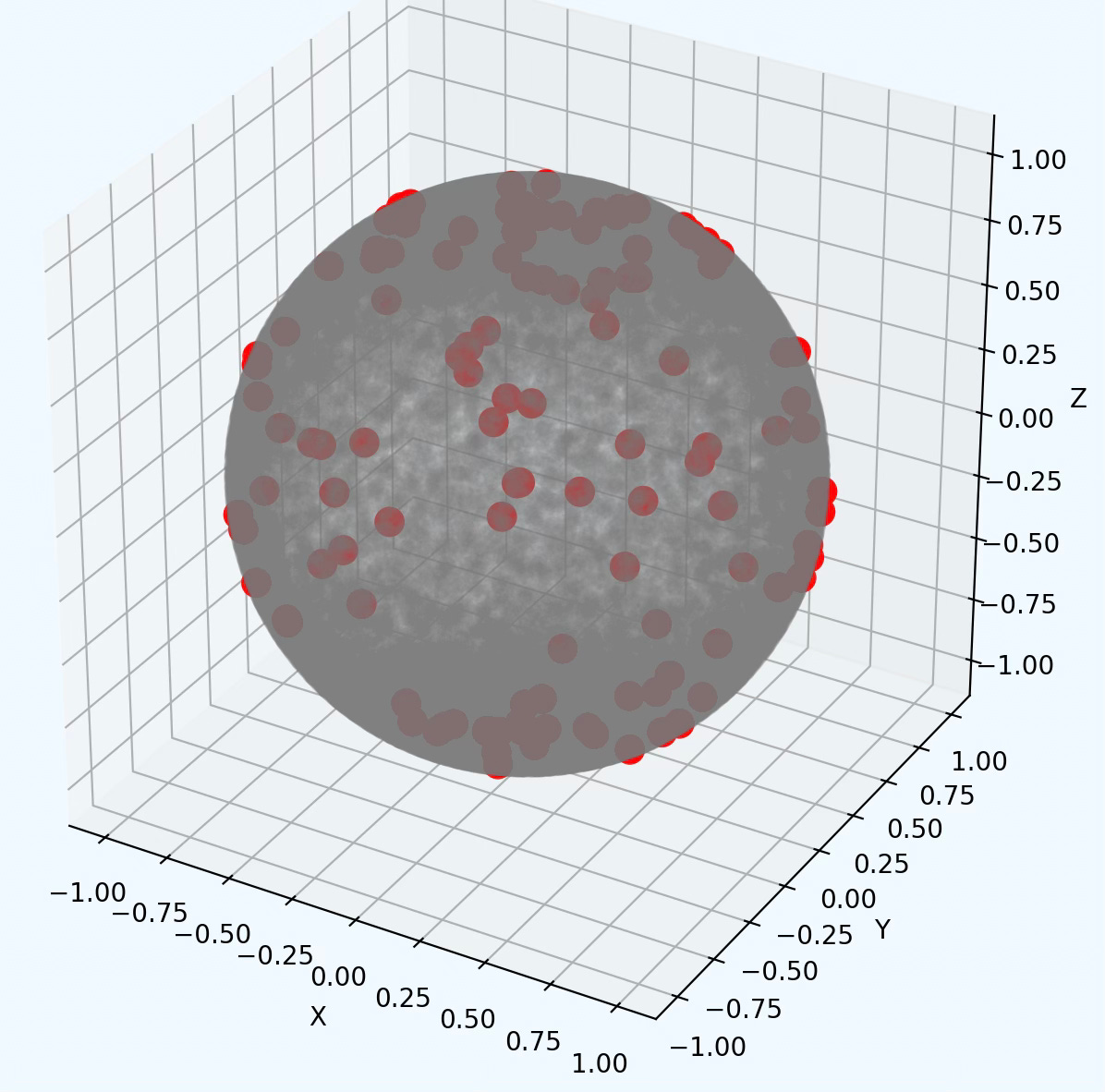
Fig. 4 Visualization of noisy data laying into a sphere

Swiss Roll

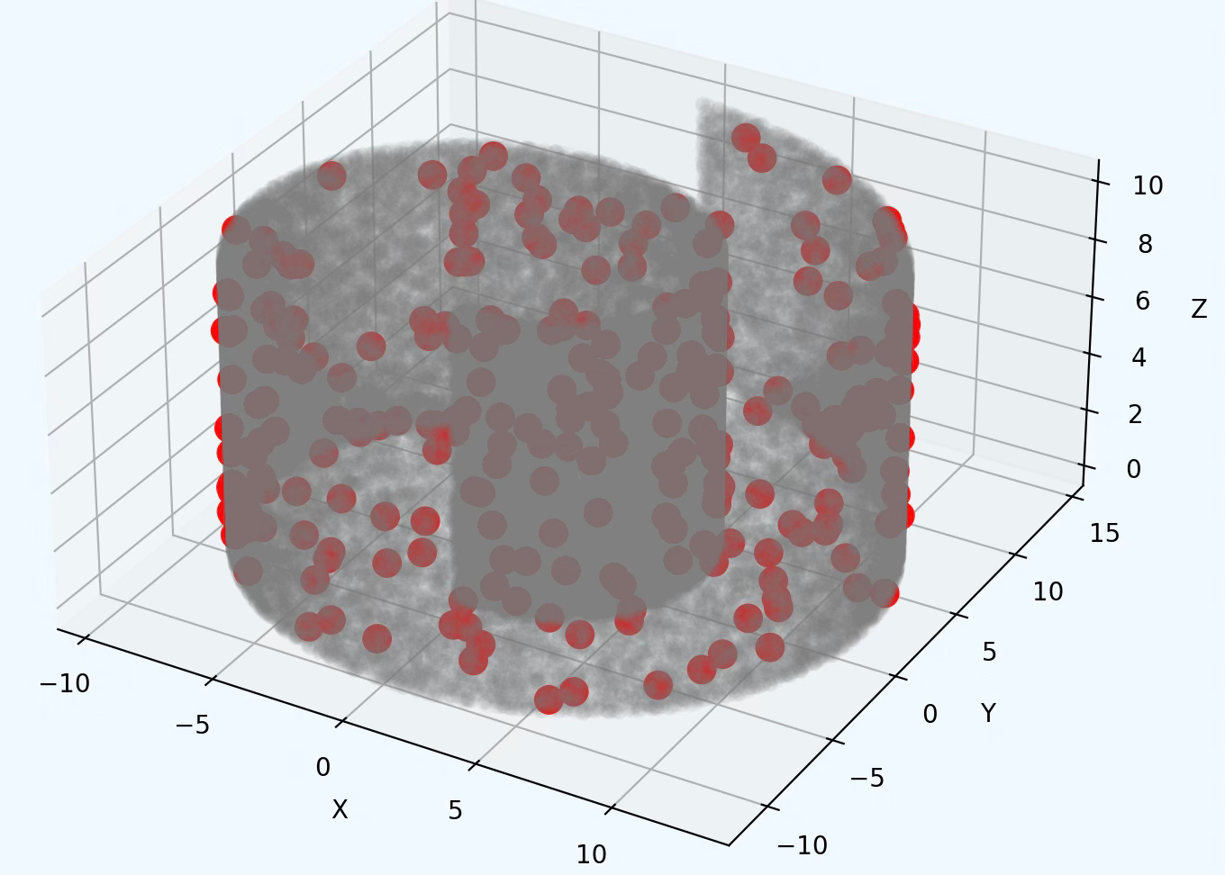
Fig. 5 Visualization of noisy data laying into a Swiss Roll

Torus

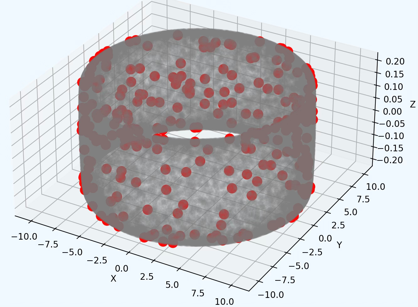
Fig. 6 Visualization of noisy data laying into a Torus manifold

🔎 For reference, I implemented the various shaped-data generator as lambdas, members of a Python enumerator ShapedDataGenerator. The lambdas are defined as

lambda: configuration parameters => data points (code snippet 1).

Examples

• Swissroll_noisy_data = SWISS_ROLL({ ‘n’: 250, ‘noise’: 0.15})

• Torus_noisy_data = TORUS({ ‘n’: 128’, ‘c’: 2, ‘a’: 0.4, ‘noise’: 0.2})

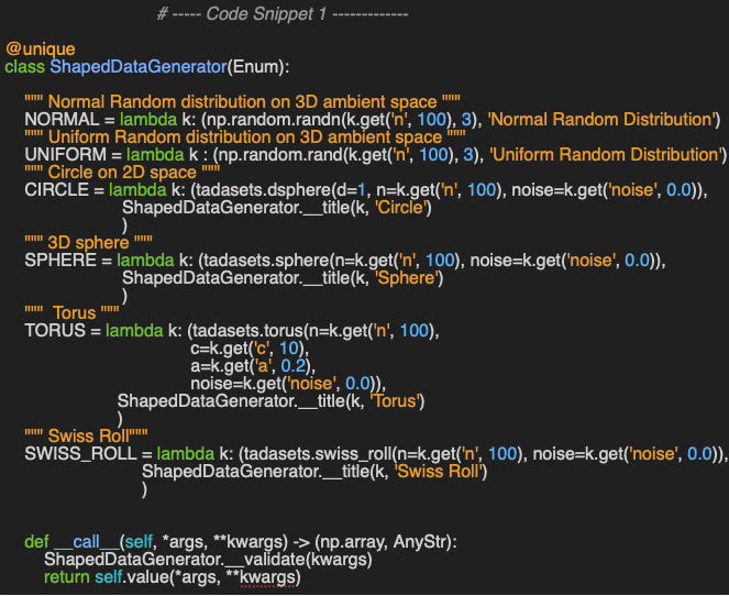
The method __call__ makes the lambda callable with configuration parameters dictionary as argument.

🔎 Persistence Diagrams

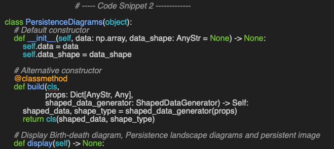
The PersistenceDiagrams class serves as a unified wrapper for all persistence diagram types, acting as an interface to BirthDeathDiagram, PersistenceImage, and PersistenceLandscape (summarized in the appendix). The default constructor initializes the noisy shape data along with its data_shape descriptor, while the alternate build constructor uses the shape descriptor and data generator introduced in the previous section (see code snippet 2).

This method - display- visualizes four different persistence diagram types, generated via the Vietoris–Rips filtration, arranged in four Matplotlib subplots (code snippet 3)

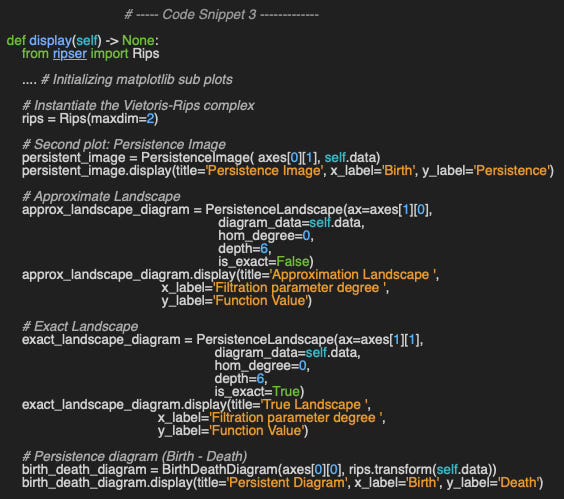
Note: Code related to the initialization of plots, not relevant to the topic, is omitted.

Let’s visualize the various persistence diagrams for the following configurations:

1. Uniformly distributed random data point in the 3D ambient space

2. Swiss-roll shaped data with 20% noise

3. Swiss-roll shaped data without noise

---

➡️ The source code for the generation of the various persistence diagrams is available at geometriclearning/topology/homology/persistence_diagrams.py and geometriclearning/topology/homology/persistence_diagrams_play.py

---

Random data points

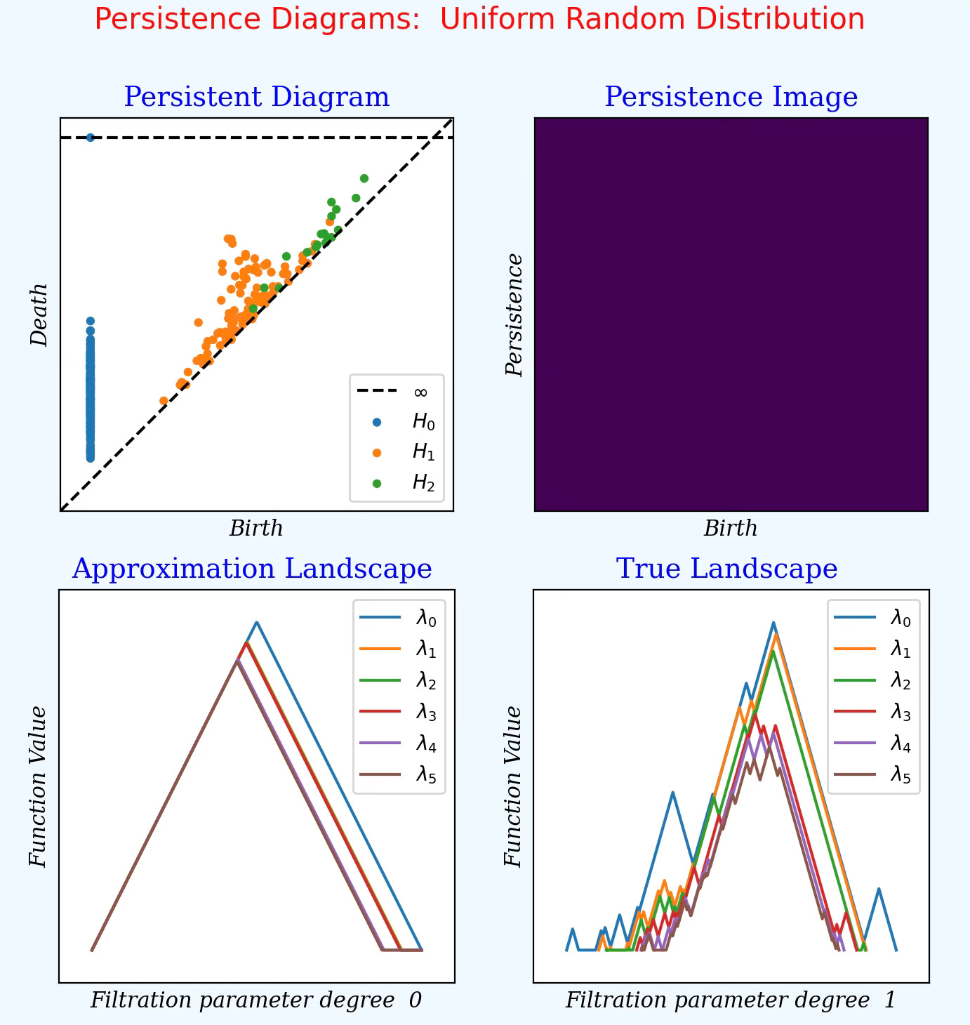
Fig. 7 Display of persistence diagrams for data point randomly distributed in 3D ambient space using a uniform distribution

Feature birth & death: As expected most of data points related to loops and voids reside in the diagonal except for the connected elements (vertices). It confirms noisy manifold with no global structure.

Persistent image: The uniform color indicated random noise with low density: no loops (H1), no voids (H2) and very ephemeral connected components (H0).

Persistence Landscape H1: The diagram shows no predominant topological feature as the lambda curves are similar

Sphere without noise

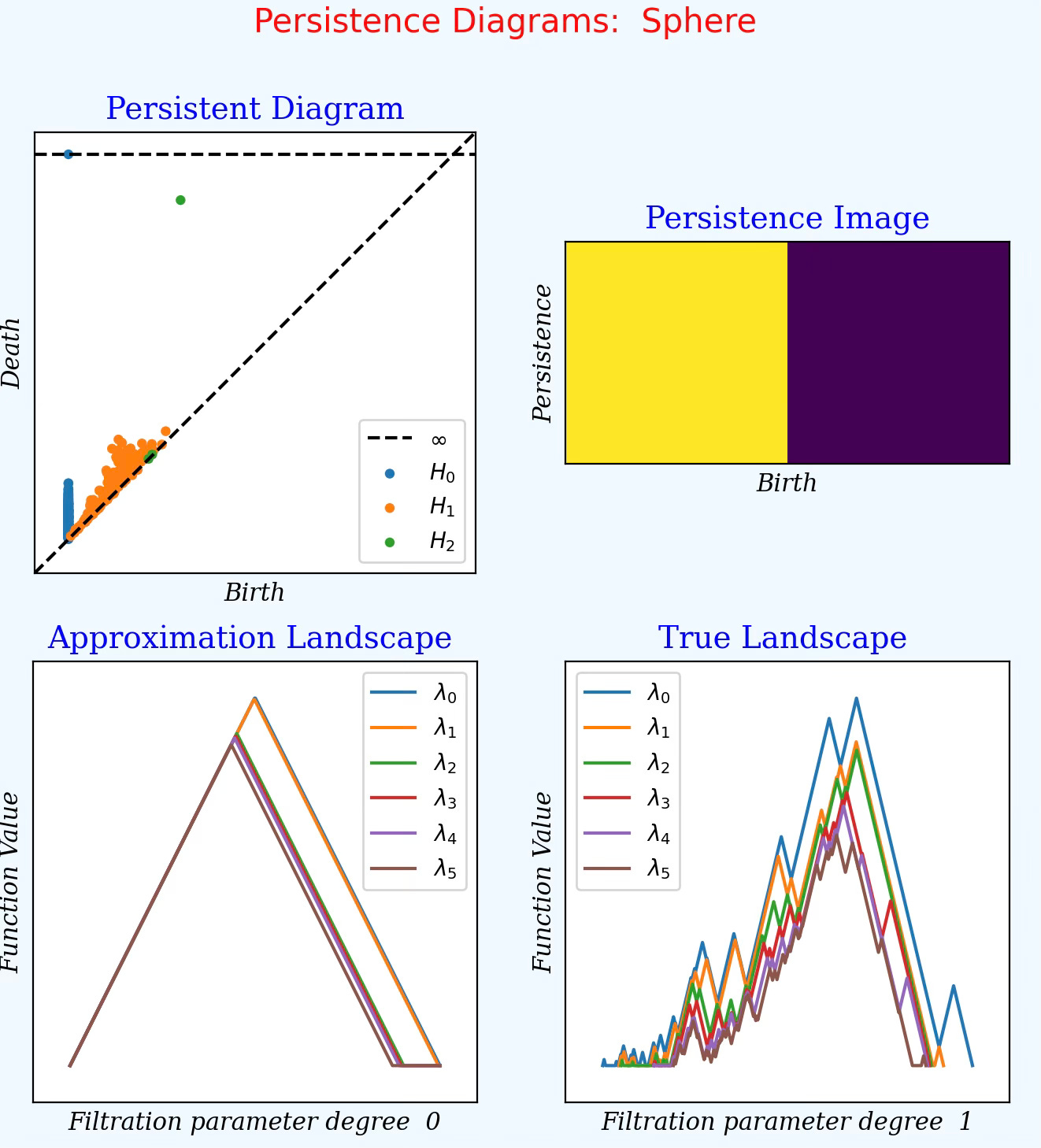
Feature birth & death: Data becomes connected into a single component (H0) with no loops (H1) and single persistent cavity (H2) confirming the detection of the sphere.

Persistent Image: The diagram confirm a very early born or detected topological features and non late born features reflecting a strong global structure - Sphere.

Persistence Landscape H0: The higher order landscapes lambda1 to lambda5 are shorted and narrower showing minimal number of isolated points with very short lifetimes.

Swiss Roll data without noise 💎

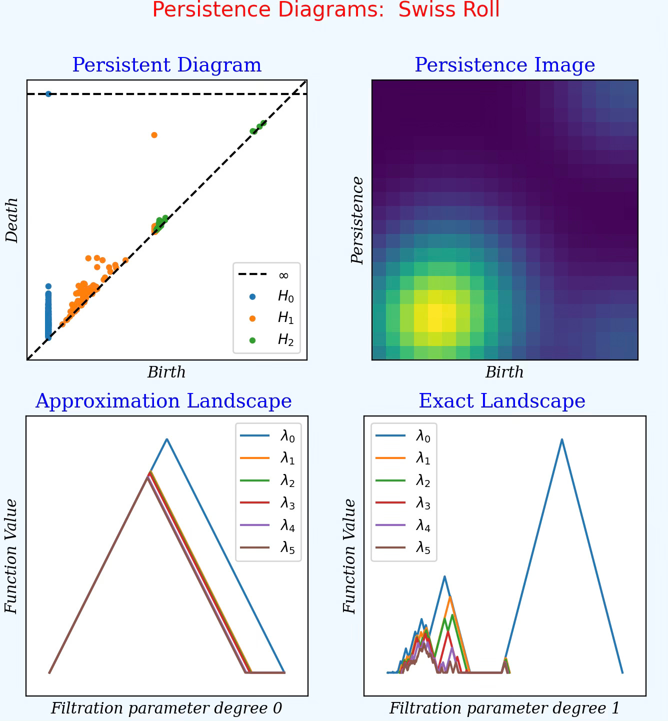
Fig. 9 Display of persistence diagrams for data point generated from a Swiss roll shape

Feature birth & death: Most loops (H1 - Orange) are very shot lived with a single outlier, indicating a single, meaningful 1-cycle (ring like structure). The H2 (green) features are weak and marginal confirming the like of a void in a Swiss roll

Persistent Image: The diagram confirms that key topological features appear early in the filtration which may reflect a recurrent mid-scale geometric pattern - Swiss roll

Persistence Landscape H0: The triangles are cleaned defined with no noise (lambda 1 to lambda 5) with a very strong dominant lambda 0 indicating that the component survives (no death). It represents a global connected structure from the data (Swiss roll).

Persistence Landscape H1: Lambda 0 is very strong, indicating a single very persistent loop that dominates all other cyclic feature, denoting a large ring or global cycle.

Torus with 15% noise 💎

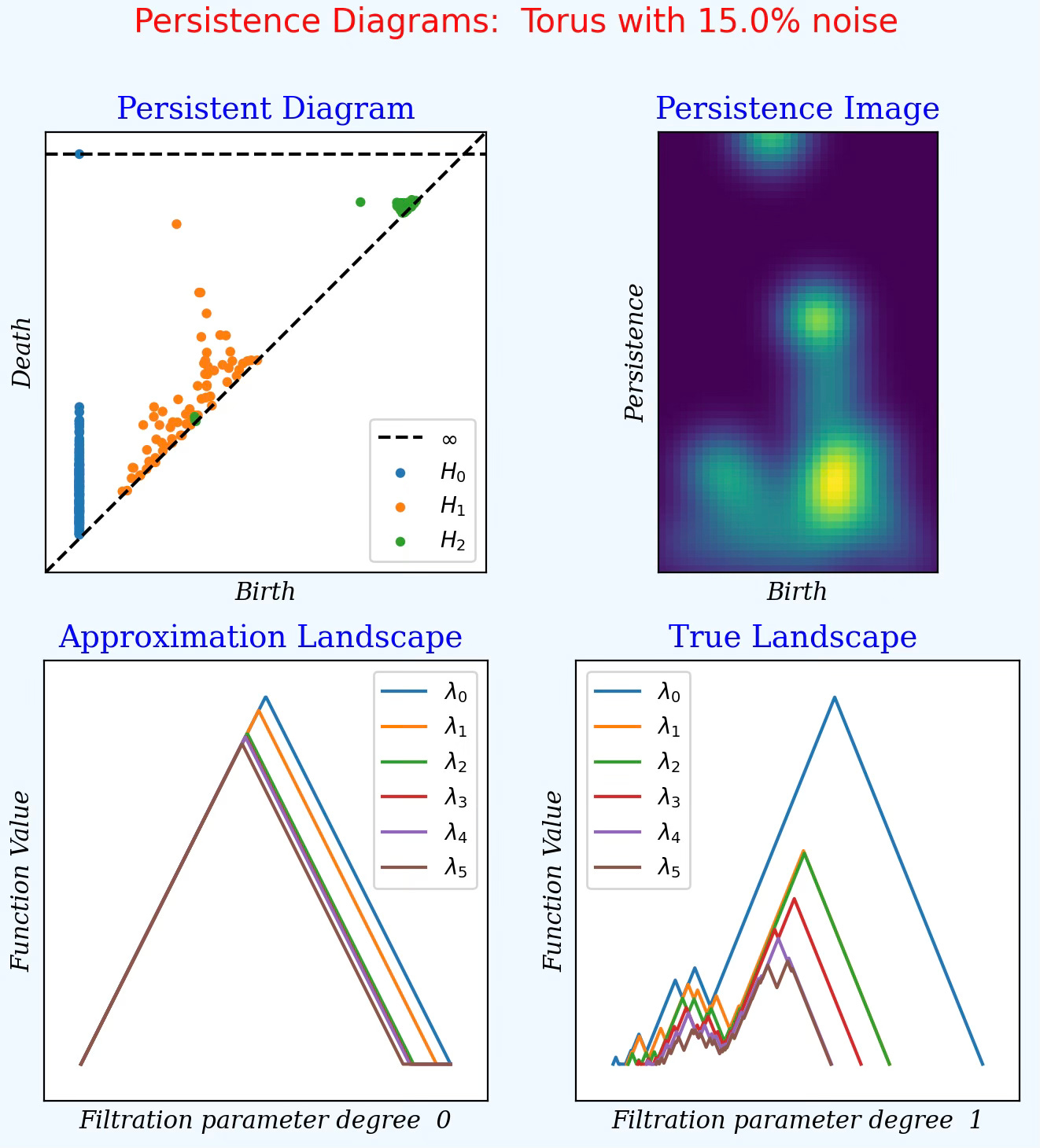
Fig. 8 Display of persistence diagrams for data point generated from a Torus shape/manifold with 15% added noise

Feature birth & death: Many components appear very early then merge quickly as the space becomes connected immediately (H0 - Blue). H1 feature indicates at least one meaningful cycle. However, a weak H2 display confirms the absence of voids.

Persistent Image: Several bright spots stacked somewhat vertically, at same birth indicates a loop where inner cycles die early while outer cycles persist. It shows a meaningful, stable, low noise topology.

Persistence Landscape H0: The diagram shows two primary connected components (lambda 0 & lambda 1) persist a lot longer than all others. This can be related to two large clusters or one main cluster along with one persistent outlier group such as a torus.

Persistence Landscape H1: Lambda 0 is somewhat strong, with declining secondary topological features with short-lived cycles.

Torus with 65% noise 💎

The objective is to evaluate the impact of noise on the extraction of topological features.

Fig. 9 Display of persistence diagrams for data point generated from a Torus shape/manifold with 65% added noise

Feature birth & death: The increased noise has very limited impact on the persistence diagram as the torus is clearly delineated manifold.

Persistent image: The bright spots are similar to ones display for the same torus with 15% noise. The ‘hazy cloud’ appearance reflects the increase scale of the noise.

Persistence Landscapes: The substantial increase in noise level from the previous configuration reduces the gap between the two primary components (lambda0 and lambda1) reflecting the less stable filtration process.

🧠 Key Takeaways 💎

✅ Working with shaped data augmented by noise is an effective way to study persistence diagrams.
✅ The birth–death (persistence) diagram acts as a topological fingerprint of the underlying data geometry.
✅ Persistence images transform these diagrams into fixed-size numerical grids that can be directly used as feature vectors in machine-learning models.
✅ Persistence landscapes map persistence diagrams to collections of functions (λkλk​) that retain essential topological information while enabling statistical analysis.
✅ Scikit-learn TDA provides a unified interface to specialized Python libraries for persistent homology, making it one of the most convenient tools for generating and manipulating persistence diagrams.

---

📘 References

1. Topological Methods in Machine Learning B. COSKUNUZER,, CÜNEYT GÜRCAN AKÇORA, 2024

2. Demystifying the Math of Geometric Deep Learning - Topology Hands-on Geometric Deep Learning, 2025

3. From Nodes to Complexes: A Guide to Topological Deep Learning Hands-on Geometric Deep Learning, 2025

4. Exploring Simplicial Complexes for Deep Learning: Concepts to Code Hands-on Geometric Deep Learning, 2025

5. Persistent homology: a step-by-step introduction for newcomers U. Fugacci, S. Scaramuccia, F. Luricich, L. De Floriani - Smart Tools and Apps in Computer Graph, 2016

6. Persistent Homology: A Pedagogical Introduction with Biological Applications U. J. Kemme, C. A. Agyingi, 2025

7. Barcodes: The Persistent Topology of Data R. Ghrist, 2007

8. Scitkit-Learn TDA 1.1.1 Documentation

9. ripser.py documentation

🛠️ Exercises 💎

• Q1: What role do persistence images play in topological data analysis?

• Q2: How persistence is computed?

• Q3: How does noise affect persistence landscapes?

• Q4: How are noisy data points reflected in a birth–death (persistence) diagram?

• Q5: What does the persistence image of a uniformly random dataset look like?

• Q6: Can you implement a subclass of PersistenceDiagramType defined in Appendix to visualize persistence landscapes - using ripser and persim packages?

Answers

🧩 Appendix 💎

Abstract base class to plot a persistence diagram

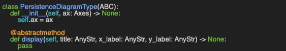
Class to plot persistence diagram (birth and death of topological features (e.g.. simplices).

---

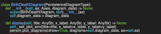
➡️ The implementation of persistent image and persistence landscape is available at geometriclearning/topology/homology/persistence_diagram_type.py

---

💬 News & Reviews 💎

This section focuses on news and reviews of papers pertaining to geometric deep learning and its related disciplines.

Paper Review Mathematical Foundations of Geometric Deep Learning Haitz Saez de Ocariz Borde, Michael Bronstein - University of Oxford, 2025

---

An excellent and comprehensive review of the mathematics underpinning Geometric Deep Learning (GDL) by two prominent experts (geometricdeeplearning.com/ for more details). Although the exposition is rigorous, it remains accessible to non-experts by clearly introducing core ideas from differential and algebraic topology.

The foundations are organized into seven categories; highlights include: foundational building blocks for deep learning (sets, maps, vector spaces) followed by norms and metric spaces; vector fields, differential operators, and gradient descent; key concepts in differential geometry; L2 function and Hilbert spaces; spectral analysis (eigenvalues/eigenfunctions and Fourier series); and a concluding overview of graph theory.

Notable gems: the role of symmetries—Invariance/Equivariance—in the bias–variance trade-off (p. 10), metrics in GDL (p. 22), and embedding latent representations into manifolds (p. 46).

---

Reader classification rating

• ⭐ Beginner: Getting started - no knowledge of the topic

• ⭐⭐ Novice: Foundational concepts - basic familiarity with the topic

• ⭐⭐⭐ Intermediate: Hands-on understanding - Prior exposure, ready to dive into core methods

• ⭐⭐⭐⭐ Advanced: Applied expertise - Research oriented, theoretical and deep application

• ⭐⭐⭐⭐⭐ Expert: Research , thought-leader level - formal proofs and cutting-edge methods.

Share the next topic you’d like me to tackle.

Patrick Nicolas is a software and data engineering veteran with 30 years of experience in architecture, machine learning, and a focus on geometric learning. He writes and consults on Geometric Deep Learning, drawing on prior roles in both hands-on development and technical leadership. He is the author of Scala for Machine Learning(Packt, ISBN 978-1-78712-238-3) and the newsletter Geometric Learning in Python on LinkedIn.