

Graphs Reimagined: The Power of Cell Complexes
Expertise Level ⭐⭐⭐

— Cell complexes extend simplicial complexes into a more general framework for higher-order network modeling, gaining particular attention for their close relationship with algebraic topology, topological data analysis and deep learning.
Table of contents
🎯 Why this matters
Purpose: This article marks the third part of our Topological Deep Learning series [refs. 1, 2]. While cell complexes are less familiar and less frequently used than simplicial complexes, they offer a powerful and flexible framework for representing geometric relationships beyond basic shapes.
Audience: Data scientists and machine learning engineers interested in topological or geometric deep learning, particularly in modeling higher-order relationships within graphs.
Value: Explore the fundamental properties of cell complexes through hands-on exercises using the TopoNetX library.
🎨 Modeling & Design Principles
Overview
In algebraic topology, cell complexes (or CW complexes) represent objects of flexible shape which are built out of basic ball-shaped building blocks (cells) of arbitrary dimension. Cells of different dimensions are rigidly related. For example, an area is enclosed by lines, which in turn are enclosed by points. This rigid structure describes the underlying topology [ref 3].
Cell complex can be used as an alternative to Graph Neural Network when data modeling requires high-order relationships [ref 4].
Cell Complexes
A cell complex is a broad, intuitive concept describing a space built from basic building blocks called cells (points, line segments, polygons, disks, etc.) that are glued together along their boundaries.
Each k-cell is homeomorphic to an open k-dimensional ball B(k)
The attaching maps describe how each higher-dimensional cell is connected to the lower-dimensional skeleton.
The main goal is to represent spaces piecewise, using discrete, combinatorial components (cells).
Example:
A triangle can be seen as a 2D cell complex built from one 2-cell (the interior), three 1-cells (edges), and three 0-cells (vertices).
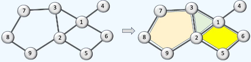
Fig. 1 Illustration comparing a graph with a 2-dimensional cell complex
A cell complex (like a simplicial or combinatorial complex) is built from cells of different dimensions:
0-cells: vertices
1-cells: edges
2-cells: faces
3-cells: volumes, etc.
Incidence Matrices
The Incidence Matrix specifies encoding of relationship between a k-dimensional and (k-1)-dimensional simplices (nodes, edges, cells={triangle, rectangle, hexagon, disk,} in a cell complex.
Rank 0: The incidence matrix of rank 1 is simply the list of node indices
Rank 1: The rank-1 matrix for directed edges between xi and xj nodes, [xi, xj] is computed as.
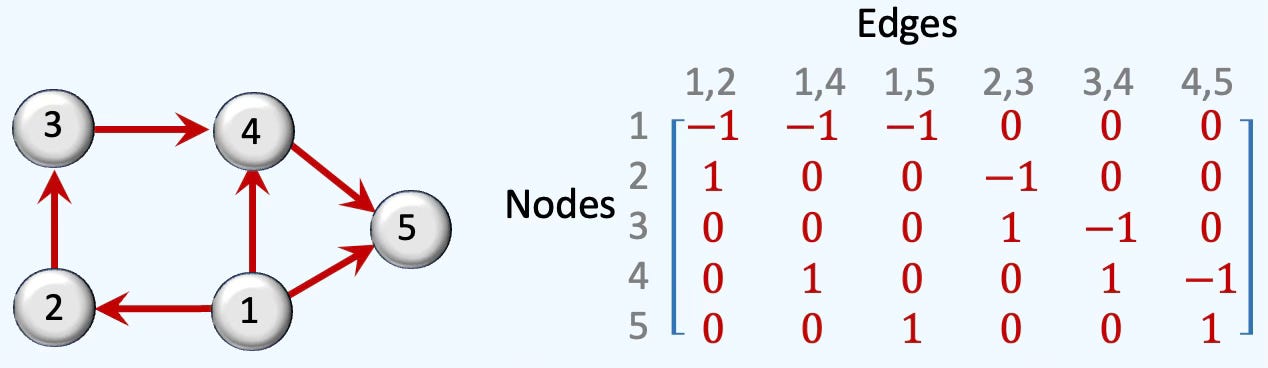
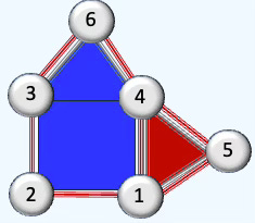
Fig. 2 Illustration of rank-1 boundary matrix of a 5-nodes cell complex
Rank 2: For a face [xi, xj, xk] with nodes xi, xj and xk and edges [xi, xj], [xi, xk] and [xj, xk].
The incidence matrix is defined as
There are only two columns in the matrix representing a triangle and a square.
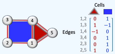
Fig. 3 Illustration of rank-2 boundary matrix of a 5-nodes, 1-cell cell complex
Adjacency & Coadjacency
Adjacency can be defined as a relation between cells of the same dimension that shared a lower-dimension boundary (e.g., 2 edges share a node or 2 cell rank 2/faces share an edge).
Given an incidence matrix B[k] mapping k-cells into (k-1)-cells:
Coadjacency defines the relation between cells of the same dimension that share the next higher-dimensional co-boundary (e.g. two edges belong to the same face/cell rank 2)
Given an incidence matrix B[k] mapping k-cells into (k+1)-cells
Laplacians
In graphs and other topological domains, the Laplacian matrix is derived from the degree and adjacency matrices. It acts as a discrete version of the Laplace operator for graph data and forms the mathematical basis of spectral clustering [refs 5, 6]
The Simplicial Laplacians are described in details in the following section of a previous article: Exploring Simplicial Complexes for Deep Learning: Concepts to Code - Simplicial Laplacians
As a reminder, the following Laplacian matrices generalize the graph Laplacian to higher-dimensional simplicial complexes. Their purposes are
Generalization of the diffusion & message passing scheme
Capture higher-order dependencies (Boundaries and Co-boundaries)
Support convolution operations in Spectral Simplicial Neural Networks
Encoding of topological features such holes or cycles.
The Upper-Laplacian (a.k.a. Up-Laplacian) is a key operator in simplicial homology and Hodge theory, defined for simplicial complexes to generalize the notion of graph Laplacians to higher-order structures. The Up-Laplacian captures the influence of higher-dimensional simplices (e.g., triangles) on a given k-simplex. It reflects how k-simplices are stitched together into higher-dimensional structures.
The Down-Laplacian (a.k.a. Low-Laplacian) is similar to the Up-Laplacian except that the boundary operator projects k-simplices to (k-1) faces. It quantifies how k-simplex is influence by its lower-dimensional faces with the following mathematical definition:
The UP and DOWN Laplacians we just introduced can be combined to generate the Hodge Laplacian. The Hodge Laplacian for simplicial complexes is a generalization of the graph Laplacian to higher-order structures like triangles, tetrahedra, etc. It plays a central role in topological signal processing, Topological Deep Learning, and Hodge theory. The Hodge Laplacian plays a central role in Simplicial Neural Networks (SNNs) by enabling message passing across simplices of different dimensions (nodes, edges, faces, etc.), while preserving the topological structure of the data. .
For a simplicial complex, the Hodge Laplacian Δk at dimension k is defined as:
However, the cell complex differs from simplicial complex by the definition of boundary.
The boundary operator for simplicial complex is explicit, combinatorial and its incidence matrix has binary values (+/- 1), and therefore easy to compute
The boundary operator for cell complex is defined by how the boundary is mapped (k-Cell to lower skeleton). Boundaries may not be uniform or be curved and complex. The computation of the Laplacian may require computation of cell adjacency and face orientation).
Closure-Weak (CW) Complexes
Closure-Weak (CW) complexes are the standard framework in algebraic topology because they guarantee good Homotopy and Homology properties [ref 7].
A CW complex (for Closure–Weak topology) is a specific type of cell complex introduced by J. H. C. Whitehead. It formalizes the idea of building spaces from cells in a rigorous topological way, satisfying two conditions:
Closure-Finiteness (C): The closure of each cell intersects only finitely many other cells.
Weak Topology (W): A subset is closed if its intersection with the closure of every cell is closed.
📚TopoNetX
TopoNetX provides tools for constructing and performing computations on topological domains. It supports operations on nodes, edges, and higher-order cells, and includes functionality for computing incidence matrices, (co)adjacency matrices, and Hodge Laplacians [refs 8 & 9]
The package is structured into five main modules:
classes: Wrapping classes for the topological domains such as simplicial complexes
algorithms: Computation of shortest cells walks, Hodge Laplacian and spectrum
transform: Lifting graphs to Cell, Simplicial Complexes and Delaunay triangulation.
datasets: PyTorch Geometric graph dataset and Stanford mesh data
generators: Generation of random simplicial and cell complexes
As expected, TopoNetX accommodates four types of topological domains:
Simplicial Complexes
Cell Complexes
Combinatorial Complexes
Colored Hypergraphs
📌 There are two other packages in TopoX suite:
TopoEmbedX extends TopoNetX by enabling representation learning across all five supported topological domains. It provides a unified API that allows embedding of simplicial, cellular, combinatorial, hypergraph, and path-based structures within a single framework.
TopoModelX is a Python library for topological deep learning that offers efficient tools for implementing topological neural networks and higher-order message-passing architectures.
Installation with dependencies
pip install toponetx topomodelx topoembedx
pip install torch-scatter torch-sparse -f data.pyg.org
⚠️
The TopoNetX implementation for Cell Complex is limited to 2-dimension contrary to the Simplicial complex
Latest version of PyTorch may not be compatible with torch-scatter or troch-sparse. Version 2.1 or earlier is recommended
⚙️ Hands‑on with Python
Environment
Libraries: Python 3.11.8, Numpy 2.3.4, TopoNetX 0.2.0
Source code: geometriclearning/topology/cell/featured_cell_complex.py
Evaluation code: geometriclearning/play/featured_cell_complex_play.py
The source tree is organized as follows: features in python/, unit tests in tests/,and newsletter evaluation code in play/.
To enhance the readability of the algorithm implementations, we have omitted non-essential code elements like error checking, comments, exceptions, validation of class and method arguments, scoping qualifiers, and import statements.
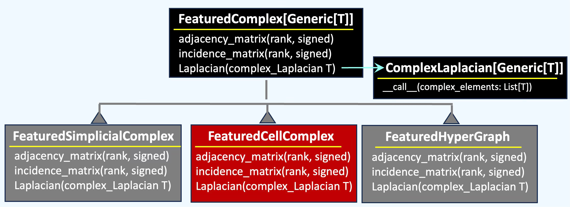
👉 We unify the functionality of multiple topological domains—Simplicial Complexes, Cell Complexes and Hypergraph—within a class hierarchy to enable systematic comparison of their behavior, from incidence matrices to Hodge Laplacians.
Featured Cell
There are two option to assign features to a cell.
Specify attribute for Cell using TopoNetX views
Assigning manually a feature vector to a cell
Setting cell attributes
This approach relies on the CellView, NodeView and EdgeView classes of TopoNetX. The protocol to assign feature keys and values to each individual cell is similar to creating a key-value pair in a dictionary as described in the follow code snippet
# Create a TopoNetX Cell complex
cx = tnx.CellComplex(cells)
# Assign a key, value to a cell identify by its tuple of
# node indices.
cx.cells[(1,2)][feature_key_1] = feature_value_1
cx.cells[(2,3)][feature_key_2] = feature_value_2
....

feature_value = cx.cells[(1, 2)][feature_key_1]
The appendix contains an example on how to assign features to a cell using TopoNetX views.
Assigning a feature vector
In this second option, we associated an optional feature vector to a cell element as a node, edge, polygon. A featured cell element is defined by its
features: An optional feature vector associated with a cell
cell: A cell with elements (indices) and rank
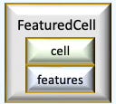
Fig. 4 Attributes of a featured cell
... and implemented in the class FeaturedCell
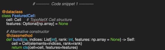
\The build class method serves as an alternative constructor that creates a TopoNetX cell from its indices and specified rank.
🔎 Setup
The class FeaturedCellComplex wraps some of the functionality of cell complex such as incidence or Laplacian matrices.
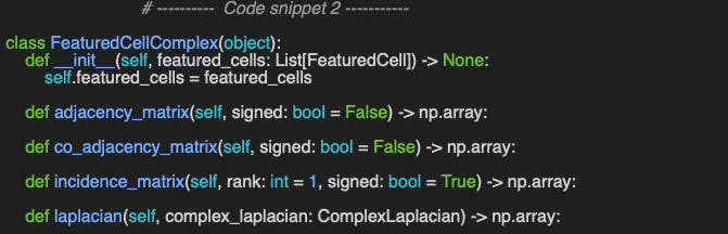
⚠️ 3-Cells - volumes attached to 2D surfaces are not supported in TopoNetX library
🔎 Adjacency & Incidence
We begin by evaluating how to extract the adjacency matrix. TopoNetX provides a general-purpose function that computes adjacency for any rank—whether for nodes, edges, or faces.
The following example - method adjacency_matrix - shows a simple and efficient computation of the rank-1 adjacency matrix.
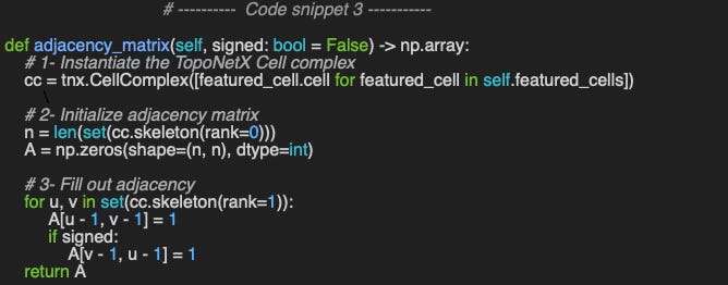
📌 The implementation of the adjacency matrix, is code snippet 3, is specific to graph (node vs. node). TopoNetX support the computation of a more generic adjacency matrix of rank > 1 using the method CellComplex.adjacency_matrix.
We define the cell simplex using the edges elements (2-node indices), edges and rank 2 cells (3/4 node indices) cells_2. The featured cell complex defined in this example is used across the entire article.
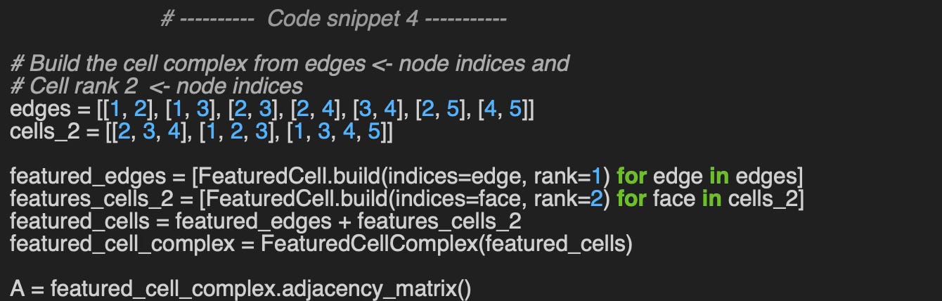
Output:
Adjacency Matrix rank 1
[[0 1 1 0 1]
 [0 0 1 1 1]
 [0 0 0 1 0]
 [0 0 0 0 1]
 [0 0 0 0 0]]
Next. let’s compute the co-adjacency matrix as illustrated in the code snippet 5.
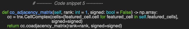
Output
CoAdjacency Matrix
  (5, 0)	1.0
  (4, 0)	1.0
  (3, 0)	1.0
  (2, 0)	1.0
  (1, 0)	1.0
  (0, 0)	0.0
  (6, 1)	1.0
  (3, 1)	1.0
         ...
  (5, 7)	1.0
  (2, 7)	1.0
  (7, 7)	0.0
  (6, 7)	1.0
  (4, 7)	1.0
The computation of the incidence matrix (see Code Snippet 6) requires specifying the cell rank and whether the cells are signed (e.g., in a directed graph). This implementation utilizes the CellComplex.incidence_matrix method from TopoNetX.
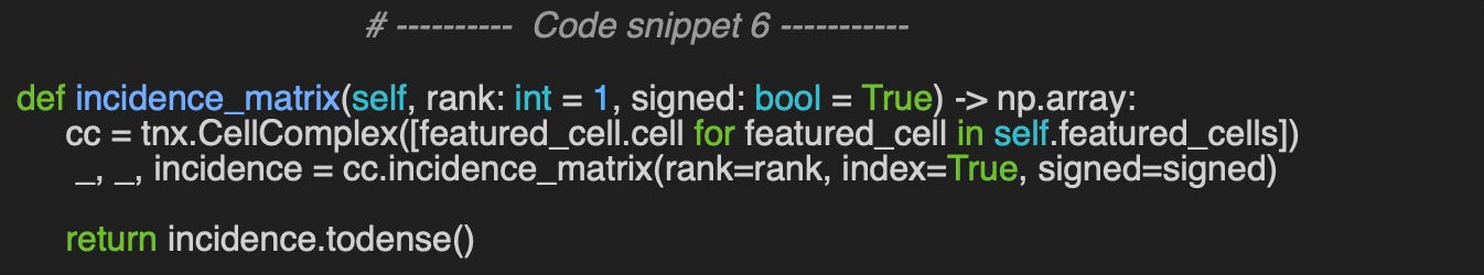
Using the sample example of cell complex configuration specified in code snippet 4 …
Output:
Incidence Matrix
[[-1. -1. -1.  0.  0.  0.  0.  0.]
 [ 1.  0.  0. -1. -1. -1.  0.  0.]
 [ 0.  1.  0.  1.  0.  0. -1.  0.]
 [ 0.  0.  0.  0.  1.  0.  1. -1.]
 [ 0.  0.  1.  0.  0.  1.  0.  1.]]
🔎 Laplacian Matrices
The final and most critical stage of our evaluation focuses on computing Laplacian matrices for cell complexes. We employed the generic ComplexLaplacian class, parameterized by the type of cell descriptor CellDescriptor: SimplexType - List of node indices or CellType. Defined previously [ref ] and reproduced in Code Snippet 8, this class supports all Laplacian variants (rank 0–2, Up/Down/Hodge).
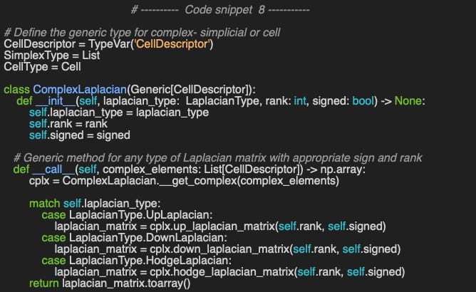
We define the type of Laplacian - laplacian_type as an enumerator
Let’ compute the Up-Laplacian for rank 1, Down-Laplacian for rank 2 and Hodge-Laplacian for rank 0, 1 & 2.
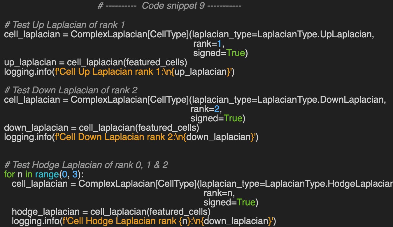
Output
Cell Up Laplacian rank 1:
[[ 1. -1.  0.  1.  0.  0.  0.  0.]
 [-1.  2. -1. -1.  0.  0.  1.  1.]
 [ 0. -1.  1.  0.  0.  0. -1. -1.]
 [ 1. -1.  0.  2. -1.  0.  1.  0.]
 [ 0.  0.  0. -1.  1.  0. -1.  0.]
 [ 0.  0.  0.  0.  0.  0.  0.  0.]
 [ 0.  1. -1.  1. -1.  0.  2.  1.]
 [ 0.  1. -1.  0.  0.  0.  1.  1.]]
Cell Down Laplacian rank 2:
[[ 0.  0.  0.  0.  0.  0.  0.  0.  0.  0.]
 [ 0.  0.  0.  0.  0.  0.  0.  0.  0.  0.]
 [ 0.  0.  0.  0.  0.  0.  0.  0.  0.  0.]
 [ 0.  0.  0.  0.  0.  0.  0.  0.  0.  0.]
 [ 0.  0.  0.  0.  0.  0.  0.  0.  0.  0.]
 [ 0.  0.  0.  0.  0.  0.  0.  0.  0.  0.]
 [ 0.  0.  0.  0.  0.  0.  0.  0.  0.  0.]
 [ 0.  0.  0.  0.  0.  0.  0.  3.  1.  1.]
 [ 0.  0.  0.  0.  0.  0.  0.  1.  3. -1.]
 [ 0.  0.  0.  0.  0.  0.  0.  1. -1.  4.]]
Cell Hodge Laplacian rank 0:
[[ 3. -1. -1.  0. -1.]
 [-1.  4. -1. -1. -1.]
 [-1. -1.  3. -1.  0.]
 [ 0. -1. -1.  3. -1.]
 [-1. -1.  0. -1.  3.]]
Cell Hodge Laplacian rank 1:
[[ 3.  0.  1.  0. -1. -1.  0.  0.]
 [ 0.  4.  0.  0.  0.  0.  0.  1.]
 [ 1.  0.  3.  0.  0.  1. -1.  0.]
 [ 0.  0.  0.  4.  0.  1.  0.  0.]
 [-1.  0.  0.  0.  3.  1.  0. -1.]
 [-1.  0.  1.  1.  1.  2.  0.  1.]
 [ 0.  0. -1.  0.  0.  0.  4.  0.]
 [ 0.  1.  0.  0. -1.  1.  0.  3.]]
Cell Hodge Laplacian rank 2:
[[ 0.  0.  0.  0.  0.  0.  0.  0.  0.  0.]
 [ 0.  0.  0.  0.  0.  0.  0.  0.  0.  0.]
 [ 0.  0.  0.  0.  0.  0.  0.  0.  0.  0.]
 [ 0.  0.  0.  0.  0.  0.  0.  0.  0.  0.]
 [ 0.  0.  0.  0.  0.  0.  0.  0.  0.  0.]
 [ 0.  0.  0.  0.  0.  0.  0.  0.  0.  0.]
 [ 0.  0.  0.  0.  0.  0.  0.  0.  0.  0.]
 [ 0.  0.  0.  0.  0.  0.  0.  3.  1.  1.]
 [ 0.  0.  0.  0.  0.  0.  0.  1.  3. -1.]
 [ 0.  0.  0.  0.  0.  0.  0.  1. -1.  4.]]
📌📌 Important note of simplicial and cell complexes: Given an underlying graph, the Laplacian matrices computed from a simplicial complex and from a cell complex are numerically identical in the absence of rank 2 cells or faces. They however differ with cell or simplex of rank 2 as these two complexes represent relationships and orientations among cells differently as the computation of their respective incidence matrices.
🧠 Key Takeaways
✅ Cell complexes generalize simplicial complexes by allowing ball-shaped building blocks (cells) of arbitrary dimension.
✅ A CW complex is a special case satisfying closure-finiteness and weak-topology conditions, which constrain how cells intersect.
✅ TopoNetX offers a convenient Python framework for exploring and evaluating such complexes.
✅ The Laplacians derived from cell and simplicial complexes on identical data differ numerically because of their distinct orientation and incidence definitions for higher-rank faces.
📘 References
From Nodes to Complexes: A Guide to Topological Deep Learning - Hands-on Geometric Deep Learning
Exploring Simplicial Complexes for Deep Learning: Concepts to Code - Hands-on Geometric Deep Learning, 2025
Don’t be Afraid of Cell Complexes: An Introduction from an Applied Perspective J. Hoppe, V. Grande, M. Schaub - RWTH Aachen University, 2025
Cell Complex Neural Networks Hajij, Istvan, Zamzmi, 2023
Graph Laplacian: From Basic Concepts to Modern Applications - H. Mhadi - Medium, 2025
A Gentle Introduction to the Laplacian S. Cristina - Machine Learning Mastery, 2022
CW Complex - Wikipedia
TopoX: A Suite of Python Packages for Machine Learning on Topological Domains M. Hajij et all, 2025
🛠️ Exercises
Q1: How does the computation of Laplacians differ between Cell Complexes and Simplicial Complexes?
Q2: What distinguishes Adjacency from Co-adjacency in topological complexes?
Q3: What two conditions must a cell complex satisfy to qualify as a CW complex?
Q4: How can the adjacency matrix for rank-2 cells be implemented in Python using TopoNetX?
Q5: What is the rank-1 Hodge Laplacian for the given cell complex?
💬 News & Reviews
This section focuses on news and reviews of papers pertaining to geometric deep learning and its related disciplines.
Paper Review: TopoBench: A Framework for Benchmarking Topological Deep Learning L. Telyatnikov et all, 2025
This is an overview of the open-source TopoBench as described in the paper; a fuller evaluation with coding exercises will come later.
TopoBench complements TopoX (by the same authors) and supports transformation, preprocessing, graph lifting, training, and evaluation for Topological Deep Learning (TDL) models. The pipeline is built on PyTorch Lightning to accelerate data handling—useful for many, though some may view it as a design constraint. The authors include a section on the crucial step of topological lifting (see my Substack: https://tinyurl.com/Topological-Lift )
Datasets in TopoBench span:
Graph-based sets from PyTorch Geometric (PyG) for exploring/evaluating GNNs that can be lifted to higher-order interactions (TopoBench wraps several PyG loaders).
Topological domains: simplicial/cell complexes and hypergraphs.
The library covers four common learning tasks: node classification/regression and graph classification/regression. The paper also reports a comparison of simplicial neural networks against standard GNNs (e.g., GCN, GAT, GIN) on mixed graph datasets and concludes with an ablation study on the same benchmarks.
Repository: https://github.com/geometric-intelligence/TopoBench
🧩 Appendix
Implementation of how to leverage TopoNetX CellComplex attributes and view to add features to nodes, edges and cells of a cell complex as described in Setting Cell Attributes
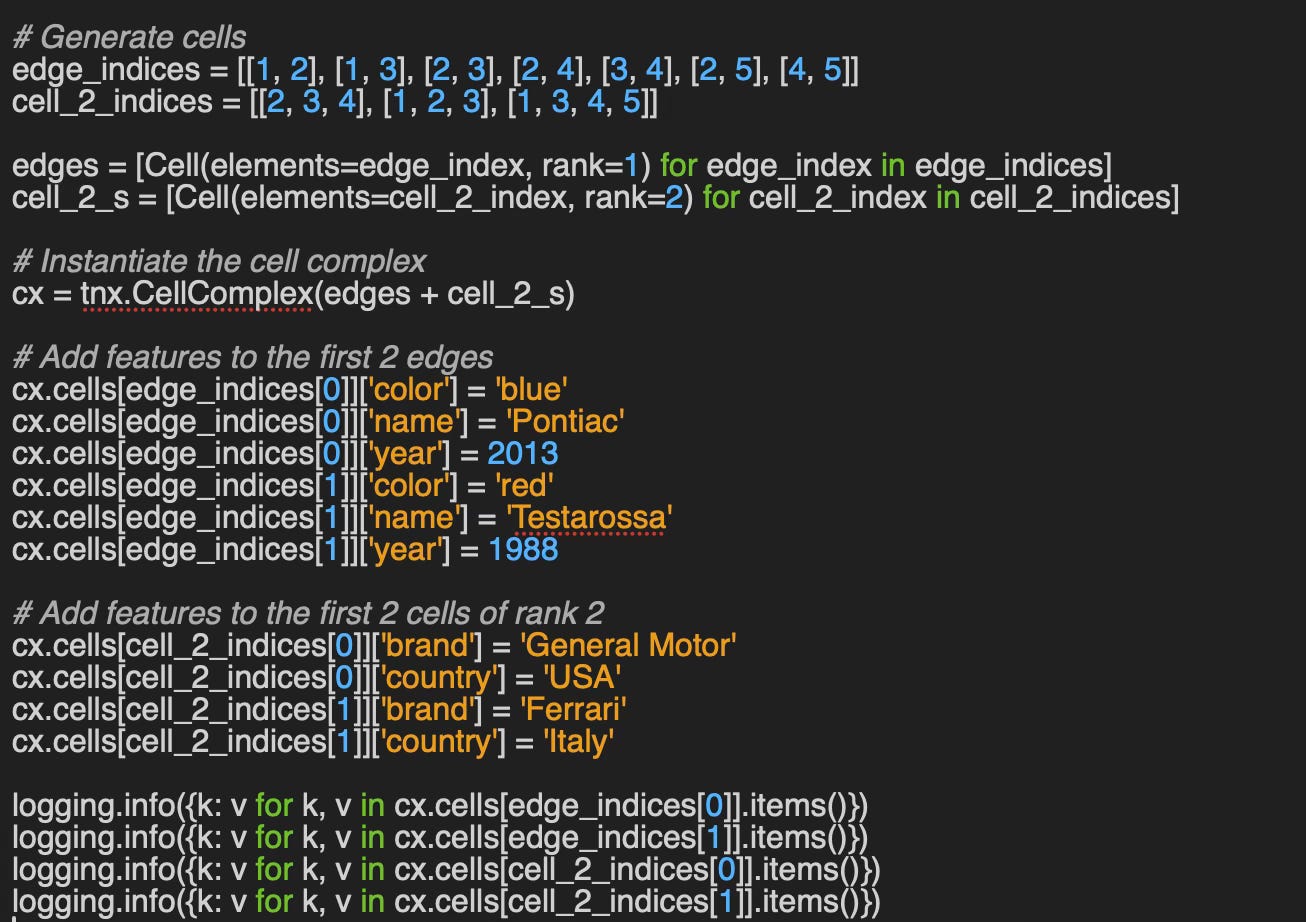
{’rank’: 1, ‘color’: ‘blue’, ‘name’: ‘Pontiac’, ‘year’: 2013}
{’rank’: 1, ‘color’: ‘red’, ‘name’: ‘Testarossa’, ‘year’: 1988}
{’rank’: 2, ‘brand’: ‘General Motor’, ‘country’: ‘USA’}
{’rank’: 2, ‘brand’: ‘Ferrari’, ‘country’: ‘Italy’}
Reader classification rating
⭐ Beginner: Getting started - no knowledge of the topic
⭐⭐ Novice: Foundational concepts - basic familiarity with the topic
⭐⭐⭐ Intermediate: Hands-on understanding - Prior exposure, ready to dive into core methods
⭐⭐⭐⭐ Advanced: Applied expertise - Research oriented, theoretical and deep application
⭐⭐⭐⭐⭐ Expert: Research , thought-leader level - formal proofs and cutting-edge methods.
Share the next topic you’d like me to tackle.
Patrick Nicolas is a software and data engineering veteran with 30 years of experience in architecture, machine learning, and a focus on geometric learning. He writes and consults on Geometric Deep Learning, drawing on prior roles in both hands-on development and technical leadership. He is the author of Scala for Machine Learning (Packt, ISBN 978-1-78712-238-3) and the newsletter Geometric Learning in Python on LinkedIn.