Decoding Neural Manifolds

Geometric Deep Learning / NeuroScience

With differential geometry and topology already playing a central role in physics, biochemistry, machine learning …, it’s no surprise that smooth manifolds have become a key tool for understanding the brain and its activity.

1. 🎯 Why this Matters

2. 🧠 Key Takeaways

3. 🌱Neural Manifolds - Basics

   🏛️ Biology

   🏛️ Dynamics of Population of Neurons

   🏛️ Spike Density Function

   🏛️ Neural Trajectory

   ⚙️ Python Environment

   ⚙️Synthetic Neural Activity

4. 🔬Neural Manifolds - Deep Dive 🔐

   🏛️ Neural Manifold Pipelines

   🏛️ Latent Representation

   ⚙️Isomap for Neural Manifold

5. 🎨 Animation 🔐

6. 📘 References 🔐

7. 🛠️ Q & A 🔐

8. 💬 Paper Review 🔐

   ---

---

👉 Patrick Nicolas is a 30-year software engineering veteran and consultant specializing in Geometric Deep Learning and World Models, author of Scala for Machine Learning, and writer of Geometric Learning in Python.

---

🎯 Why this Matters

Purpose: Structuring subjective experiences geometrically is a pre-requisite to link them to physical data and the patterns of firing neurons in the brain.

Audience: Data scientists and engineers curious about application of manifolds to represent brain activity.

Value: Develop a practical intuition for neural dynamics and latent manifolds by simulating spike trains with Poisson distributions and extracting topological structures using kernels and Isomap.

🧠 Key Takeaways

✅ Signal Generation: Neural activity is an electrochemical process where neurons communicate via discrete events known as spikes.

✅ Data Preprocessing: Raw spikes are recorded per neuron and normalized across specific time bins to ensure statistical consistency.

✅ Manifold Extraction: Neural manifolds can be derived as discrete structures via eigendecomposition of the activity matrix, or as continuous representations using convolutional methods.

✅ Signal Smoothing: Discrete spike trains are transformed into continuous temporal functions, f(t), by convolving them with Gaussian or exponential kernels.

✅ Dimensionality Reduction: The high-dimensional Hilbert space containing these functions is projected onto a low-dimensional subset, defining the neural manifold.

🌱 Neural Manifolds - Basics

---

⚠️ My knowledge in geometric learning does not make me an expert in neuroscience or biology, far from it. However, I thought it would be helpful to describe biological neuron prior to introducing neural manifolds - I hope expert readers will forgive me. Instructive references are listed at the end of this article.

---

🏛️ Biology

Biological neurons are the fundamental building blocks of the entire nervous system including the brain. They responsible for receiving, processing, and transmitting information throughout the body [ref 1].

This picture worths a thousand words …

Fig. 1 Illustration of a biological neuron

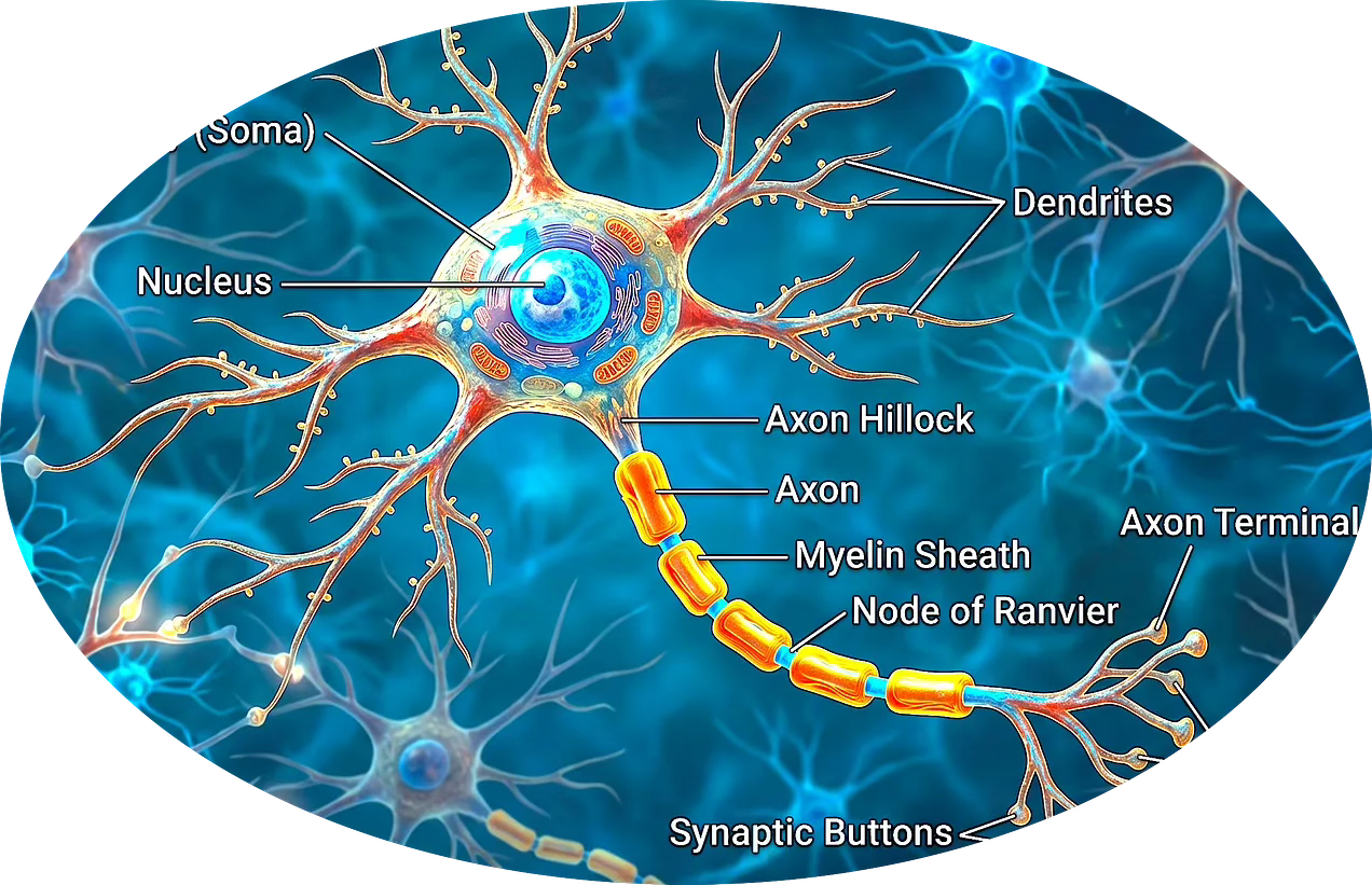
The basic functional components are:

• Dendrites: Branch-like structures extending from the cell body that act as antennas, receiving signals from other neurons.

• Soma: The metabolic center of the cell containing the nucleus and DNA, which sums up all incoming information from the dendrites.

• Axon: A long tail-like structure that carries electrical impulses (action potentials) away from the soma to other neurons, muscles, or glands.

• Axon Terminals: The end of the axon where chemical signals called neurotransmitters are released to pass the message to the next cell.

'

---

📌 Biological neurons are also called as nerve cells or neural cells

---

You may wonder how biological neurons compare with artificial neural units. Artificial neural networks are over-simplified versions of biological cell networks as illustrated in the following table.

Table 1 Basic comparison between biological and artificial neurons

Biological neurons can be categorized as Unipolar (single process extending from the body), Bipolar (one pair axon-dendrite), Multipolar (one axon - many dendrites) & Pseudo-unipolar (multiple process branches).

🏛️ Dynamics of Population of Neurons

Neural activity refers to the complex electrochemical processes by which neurons generate, and process information. For this article, I restrict the definition as the action potential or spike generated by a biological neuron.

Neural activity is obviously constrained by the properties of the physical network of neurons. These constraints reduce the neural activity patterns to low-dimensional subspace — manifold — within an high-dimensional ambient Euclidean neural space. While a population of N neurons could theoretically produce an infinite variety of firing patterns within an N-dimensional space, their actual activity is constrained to a much simpler, lower-dimensional surface [ref 2, 3, 4].

Researchers collect brain activities (neuron firing) through electrodes. The neural activity can be visualized as spikes as illustrated below:

Fig. 2 Illustration of neural activity for 4 biological neurons with a sliding time window

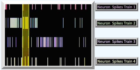
Since information is distributed across a population of neurons, it raises a fundamental question: what are the correlative or causal relationships between the spikes within that group? One approach to answering this question is to analyze the collective firing patterns across multiple neurons within a specific (sliding) time window.

---

📌 Some articles may use the term neural discharge instead of neural spikes.

---

🏛️ Spike Density Function

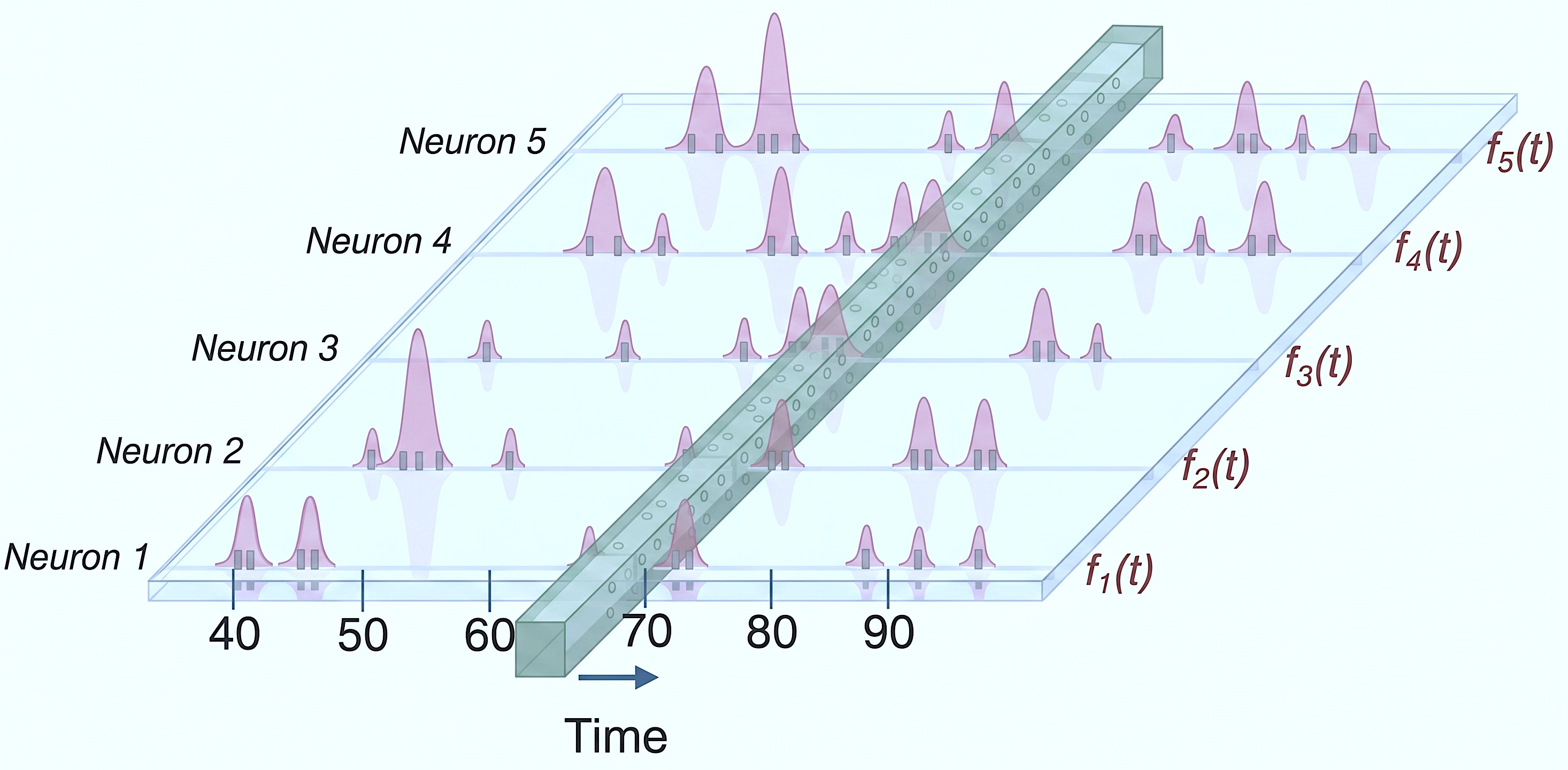
Neural manifolds are fundamentally smooth manifolds and therefore we need to convert the train of spikes associated with each neuron into a smooth function. Mathematically speaking, those spikes are Dirac delta functions and can be smoothed as Spike Density Function (SDF)

Convolution

Given a Kernel K and a spike train S, the SDF is computed as a convolution f

\(S(t)=\sum_{i=1}^{n}\delta(t - t_{i}) \ \ \ \ \ f(t)=(S*K)(t)=\int_{-\infty }^{+\infty }S(x)K(t-x)dx \)

Using an exponential kernel

\(K(x)=\begin{matrix} \alpha e^{-\alpha x} \ \ x \ge 0\\ 0 \ \ \ \ \ \ \ \ \ x \lt 0 \end{matrix} \ \ \ \ \ \ \ \ \ \ \ f(t)=\sum_{t_{i}\le t}^{}\alpha e^{-\alpha (t-t_{i})}\)

Using a Gaussian kernel

\(K(t)=\frac{1}{\sigma\sqrt{2\pi}}e^{-(\frac{t}{\sqrt{2}\sigma})^{2}} \ \ \ \ \ \ \ \ f(t)=\sum_{i=1}^{n}\frac{1}{\sigma\sqrt{2\pi}}e^{-(\frac{t-t_{i}}{\sqrt{2}\sigma})^{2}}\)

📌 There are many alternative to the exponential kernel. The exponential kernel is used in computational neuroscience because it can be computed recursively without needing to store the entire history of spikes as follows:

\(\frac{d f(t)}{dt}=\alpha \left[ S(t-f(t) \right]\)

The value of the smoothing Spike Density Function is proportional to the number of spike (neuron firing) within the time window as illustrated below:

Fig. 3 Illustration of Spike Density Function applied to the neural activity of 5 neurons

🏛️ Neural Trajectory

The next step is to represent the neural activity as a neural trajectory in the Euclidean space which dimension is equal to the number of neurons. Neural manifolds are abstraction of neural trajectories and neural dynamics as low representation of high dimensional neural activity [ref 5].

The following diagram illustrated a 2-dimensional manifold extracted from the neural activity of 3 biological neurons.

Fig. 4 Visualization of a 2 dimensional neural manifold representation of the neural activity of 3 biological neurons.

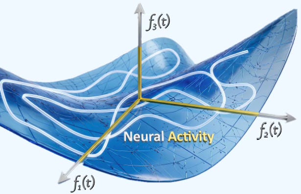
Think of a neural manifold as a mathematical map of what a group of neurons can actually do. While thousands of neurons could theoretically fire in endless combinations, their physical wiring and the task at hand force their activity onto a much simpler, low-dimensional surface. By studying these shapes of neural activity, we gain a clearer window into how the brain coordinates complex behavior.

⚙️ Python Environment

• Libraries: Python 3.12.5, Numpy 2.3.5, Matplotlib 3.10.1

• Implementation code: geometriclearning/deeplearning/model/synthetic_neural_manifold.py

• Evaluation code: geometriclearning/play/synthetic_neural_manifold_play.py

• The source tree is organized as follows: features in python/, unit tests in tests/, and newsletter evaluation code in play/.

• To enhance the readability of the algorithm implementations, we have omitted non-essential code elements like error checking, comments, exceptions, validation of class and method arguments, scoping qualifiers, and import statements.

⚙️ Synthetic Neural Activity

A neural activity can be synthetically generated by sampling a manifold embedded in the neural data space. I selected the simplest manifold S(1) or circle.

The sampling from the 1 dimension manifold (circle) at time t is implemented by the following formula.

\(\begin{matrix} x_{L}=cos(t) \\ y_{L}=sin(t) \end{matrix} \ \ \ \ \ [1]\)

Generation of the spike density function uses the Poisson distribution with the sum of square between the predicted values and the latent values

\(Poisson(k; \lambda)=\frac{\lambda^k e^{-\lambda}}{k!} \ \ \ \ \lambda = \frac{1}{2}[(\tilde{x}-x_{L})^2 + (\tilde{y}-y_{L})^2] \ \ \ \ [2]\)

🔎 Let’s wrap the generation of Neural spikes into a class, NeuralActivityGenerator. Its constructors has 4 parameters

• n_neurons: Number of neurons (dimension of the Euclidean data space)

• n_timesteps: Number of time sampling over a given period of time

• firing_rate_factor: Scaling factor for the parameter of the Poisson distribution

• velocity: Scaling factor for the time frame of the sampling, computed as n_timesteps* velocity.

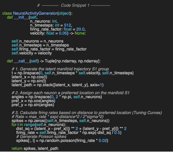
The method ‘__call__’ implements the generation of the spike trains in 3 steps:

1. Generate the latent space as a circle (S1 group) using a time line parameterized by n_timesteps - formula 1

2. Sample the circular latent space, using equidistance 2.PI/n_neurons

3. Compute the spikes train for each neural give a firing rate computed by formula 2

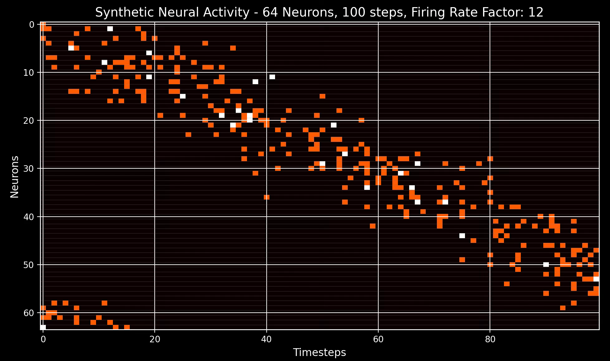
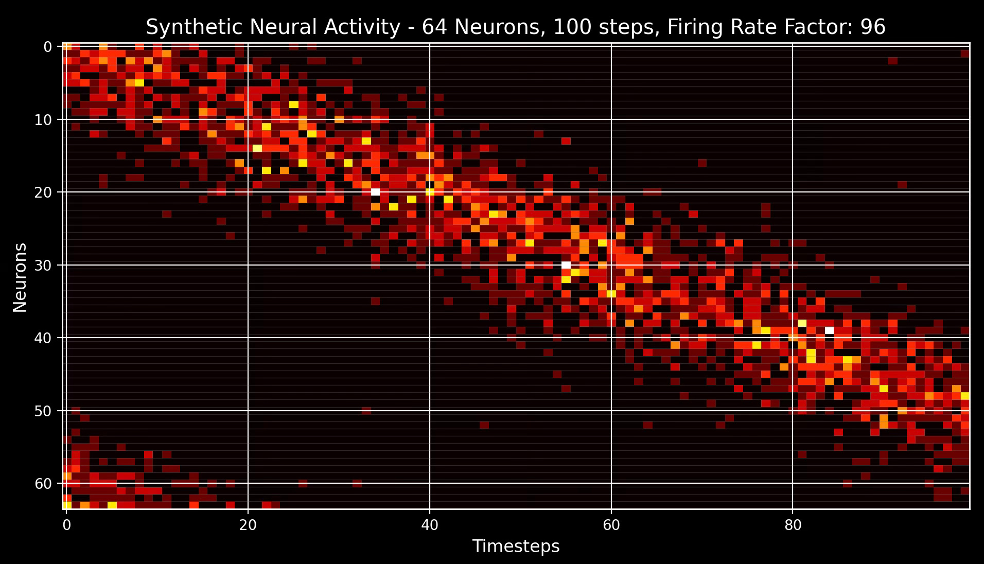
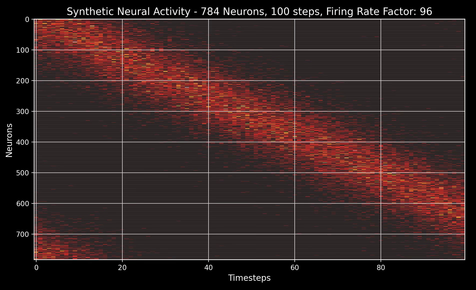
The neural activity as computed by NeuralActivityGenerator.__call__ is visualized for 64 and 784 neural and a slow vs. fast firing rate.

Fig. 6 Visualization of a synthetic neural activities of 64 neurons over 100 time steps and a firing rate factor of 12.

Fig. 7 Visualization of a synthetic neural activities of 64 neurons over 100 time steps and a firing rate factor of 96

Fig. 8 Visualization of a synthetic neural activities of 784 neurons over 100 time steps and a firing rate factor of 96

🔬 Neural Manifolds - Deep Dive 🔐

🏛️ Neural Manifold Pipelines

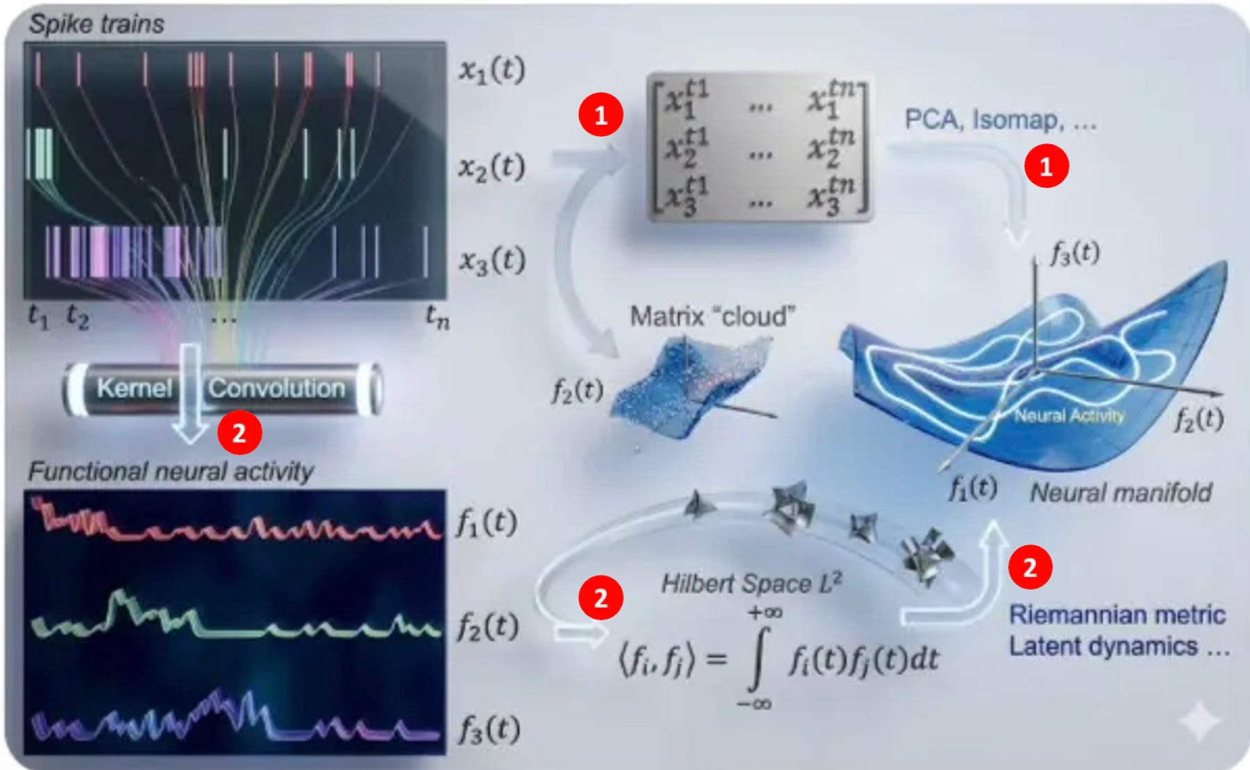
From a practical view, there are two approaches to extract neural manifold properties from neural activity of n neurons:

1. Pipeline 1: Generate a matrix n (spike trains) by m (time steps) then compute linear dimension reduction (PCA), or non-linear dimension reduction (Kernel PCA, Isomap, Laplacian Heatmap …).

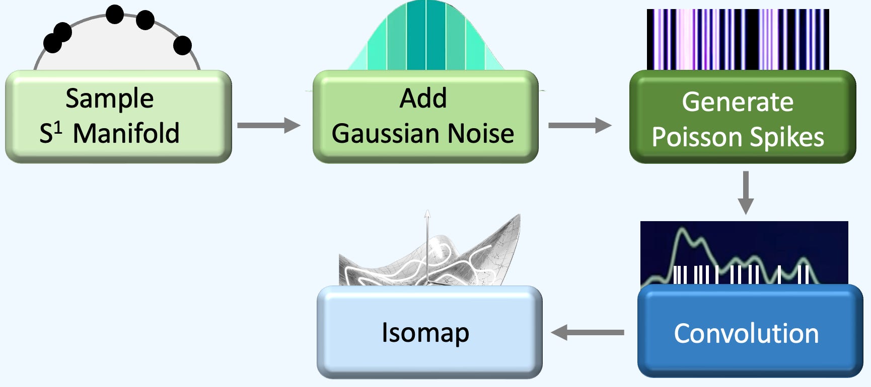
2. Pipeline 2: Convert the n spike trains into n continuous function using Gaussian convolution, resulting in a L2 Hilbert space then compute the Riemannian geometric properties such as metric, geodesic and intrinsic curvature.

Fig. 9 Visualization of the 2 pipelines to generate neural manifolds

Here is an illustration of the 5 steps of pipeline #2 to extract a neural manifold through a synthetic neural activity derived from a S1 neural manifold:

Fig. 10 Pipeline to Generate of neural manifold from neural activity sampled from S1 group using Isomap manifold learning

🏛️ Latent Representation

The section, Neural Manifold Pipelines, lists two techniques to extract the low-dimensional manifold from the neural activity. Both rely on the Isometric Features Mapping manifold learning algorithm [ref 6, 7]

Isometric Features Mapping (Isomap) is one of the non-linear manifold learning that relies on two principles:

• Isometry: The geodesic distance on the manifold is invariant under the mapping to the tangent, Euclidean space.

• Convexity: The manifold is a convex subset of the ambient Euclidean space

---

📌 The Isometric Feature Mapping (Isomap) is the nonlinear generalization of the MultiDimensional Scaling (MDS)

---

👉 The Isomap algorithm is one of the manifold learning techniques supported by Sklearn module manifold.

Isometric Feature Mapping (Isomap)

The core idea is to represent the data set (Neural Activity) as a graph, G with n data points, defined as vertices x and Euclidean distance DG as edges. For the points belonging to the neighborhood E, the weight of edges W is computed as [1]

\(D_{G_{i,j}}=W_{i,j}=|| x_{i} - x_{j}|| \ \ \ [1]\)

For points that are not immediate neighbors, the distance DG is computed along the geodesic of the manifold [2].

\(D_{G, ij} = \begin{cases} W_{ij} & \text{if } (i,j) \in E \\ 0 & \text{if } i = j \\ \infty & \text{if } (i,j) \notin E \end{cases} \ \ \ [2]\)

The geodesic distance is the shortest path distance between any sequence of vertex in G. I use the Dijkstra’s algorithm. For instance, a path through 3 nodes, i, j & k is simply computed through minimization [3]. The geodesic distance on a smooth manifold is theoretically computed by increasing the number of vertices to infinity (or weights of edges to zero) [4].

\(D_{G_{,ij}} = min (D_{G_{,ij}}, D_{G_{,ik}}+ D_{G_{,kj}}) \ \ [3] \ \ \ \ \ \ d_{M}(x_{i}, x_{j})=\lim_{n \to \infty } D_{G_{,ij}} \ \ [4]\)

Finally we apply the Multidimensional Scaling (MDS) algorithm to construct the d-dimensional embedding as follows

\(B = -\frac{1}{2}H(D_{G_{ij}})^2H \ \ \ \ \ \ \ B =V \Lambda V^{T} \ \ Eigendecomposition\)

The Eigendecomposition of the Gram, symmetric matrix B generate n eigenvalues. The Eigenvectors associated with the d « n largest eigenvalues are the Isomap embeddings.

⚙️ Isomap for Neural Manifold

I encapsulated the generation of the latent manifold in the class SyntheticNeuralManifold that takes the generation of neural activity as its only argument.

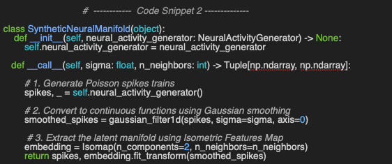
The algorithm, implemented in ‘__call__’ method, follows 3 simple steps:

1. Generate the spike trains

2. Convert the spikes train (Dirac delta) into continuous functions, for each neuron, using a Gaussian filter.

3. Apply the Isomap in 2 dimension to the array of functions.

I used Matplotlib to display the scatter plot between the 2 principal dimensions as illustrated below

Fig. 11 Visualization of a neural manifold extracted from the neural activity of 64 neurons using a Gaussian smoothing function with standard deviation 1.6 and 33 Isomap neighbors.

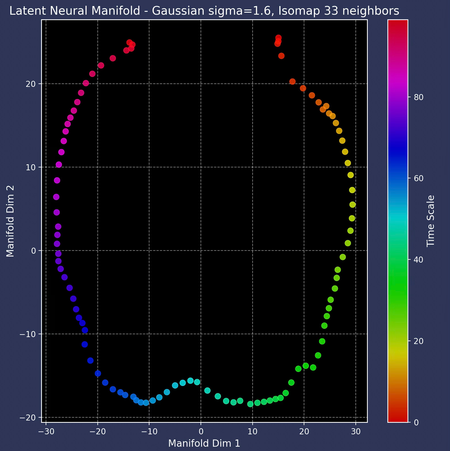
We can clearly recognize the circular trajectory of the sample S1 manifold. The resulting trajectory is distorted by the introduction of the Gaussian noise in the generation of spike train.

---

📌 Scaling neural activity down to two dimensions is challenging; it requires fine-tuning both the Gaussian filter’s standard deviation and the neighborhood function settings for every neuron.

---

🎨 Animation 🔐

The following Manim dynamic visualization illustrates the key points introduced in this article.

📘 References 🔐

1. An Introduction to Biological Neurons - Zenva, 2018

2. From sensory to perceptual manifolds: The twist of neural geometry - H. Ma, L. Jiang, T. Liu, J. Liu, 2025

3. A unifying perspective on neural manifolds and circuits for cognition - C, Langdon, M. Genkin, T. A. Engel - Nature Reviews, Neuroscience, 2023

4. Neural Manifolds for the Control of Movement - J.A. Gallego, M.G. Perich., L.E. Miller, S.A. Solla - YouTube, 2017

5. Computation and Neural Manifolds - David Barack, UC Merced - YouTube, 2023

6. Manifold Learning: Theory and Applications: -Y. Ma, Y. Fu, - CRC Press, 2012

7. Introduction to IsoMAP: Isoscapes Modeling, Analysis, and Prediction - Isoscapes, 2011

🛠️ Q & A 🔐

1️⃣ How do we formally define the neural activity?

2️⃣ Can you summarize the difference between biological and artificial neurons inter term of learning strategy and processing?

3️⃣ What is a Spike Density Function? Can you provide examples?

4️⃣ What is the purpose of Poisson distribution for generating spikes train?

5️⃣ What are the properties of Isomap that makes it particularly applicable in extracting neural manifolds?

👉 Answers

💬 News & Reviews 🔐

This section focuses on news and reviews of papers pertaining to geometric deep learning and its related disciplines.

Paper Review: Neural manifold analysis of brain circuit dynamics in health and disease - R. Mitchell-Heggs, S. Prado, G. P. Gava1, M, A. Go, S. R. Schultz, 2022

---

This is one of the most concise papers introducing Neural Manifolds in the context of health care. Neural Manifolds are low-dimensional topological structures that represent the spatiotemporal dynamics of neural activity, that is defined as spike trains (time series) of neural population.

The authors introduce Neural Manifold Learning (NML) to understand the neurobiological basis of behavior and patterns of neural population activity. NML algorithms shared the objective of dimension reduction and are categorized as linear (Principal Component Analysis), Multidimensional Scaling) and non-linear (Isomap, Locally Linear Embedding, Laplacian Eigenmaps, t-SNE, UMAP (ref: Introduction to UMAP and Probabilistic Latent Variable Models).

The selection of the most appropriate model is challenging and depends on the signal-to-noise ratio of input data. It relies on multiple trials. A Neural Network based approach such as variational auto-encoder can be a great solution in the case the resulting low-dimensional manifold is not entangled.

The authors evaluate the NML algorithms against several large-scale neural datasets related to the hippocampus and motor cortex through reconstruction of the encoded high-dimensional neural activity. They describe a parameterization method to overcome the key challenge is to estimate the intrinsic dimension of the neural manifold.

In conclusion, neural manifold learning models are a powerful toolbox to understand the coordination of population of neurons during specific behavioral tasks.

Share the next topic you’d like me to tackle.