

Hands-on Stochastic Gradient Langevin Dynamics

Although a powerful and ubiquitous optimization method, the Stochastic Gradient Descent has fundamental structural limitations that make it unsuitable for some types of complex landscapes and Bayesian inference.
The Stochastic Gradient Langevin Dynamics fills the gap between optimization and random (Monte Carlo) sampling.
🎯 Why this Matters
Purpose: Scientists have been trying to combine function optimization and random sampling to improve reliability of Bayesian inference and the minimization of the loss function in training of large models. Stochastic Gradient Langevin Dynamics (SGLD) mitigates the risk of converging to local minima by injecting Gaussian noise proportional to the square root of the learning rate, thereby facilitating global exploration of the loss landscape.
Audience: Data scientists and researchers looking to expand their understanding and evaluate alternative for Bayesian inference or training deep learning models.
Value: Learn the behavior of the Stochastic Gradient Langevin Dynamics as compared to Stochastic Gradient Descent and Adam algorithm using landscape loss function (e.g. Ackley).
🎨 Theory
Overview
The best strategy to evaluate SGLD is to compare it with optimization methods we are all familiar with - Stochastic Gradient Descent and Adam.
Gradient Descent Family
Gradient Descent (GD)
The Gradient Descent is the simplest form of optimization and a direct application of calculus. This is an iterative optimization algorithm used to minimize loss functions in machine learning.
Give a learning rate alpha, a loss function L, feature values vector x and label y
Stochastic Gradient Descent (SGD)
The vanilla Gradient Descent is notorious for slow convergence toward global minimum as it requires to process the entire datasets.
The stochastic version enables faster, highly efficient, and scalable learning for large datasets with two improvements has been made to the original Gradient Descent [ref 1]:
Selection of random training pair features-label {xi, yi}
Organizing these random training samples into mini-batch of size m
SGD is noisy but converges faster than the original Gradient Descent.
Nesterov Accelerated Gradient (NAG)
Given the momentum v, the momentum coefficient beta, the learning rate alpha and the mini-batch of size m
Nesterov acceleration changes the convergence rate of gradient descent on convex functions.
Gradient Descent: Converges at a rate of O(1/t)
Nesterov Momentum: Converges at a rate of O(1/t**2)
Adaptive Moment Estimation (ADAM)
Adam computationally efficient optimization algorithm for training deep learning models, addressing the short comings of SGD by combining the benefits of AdaGrad and RMSProp [ref 2]
It updates the learning rates for each parameter as described by the formulas below, using two momenta
First moment - similar to the mean - m (1)
Second moment or adjusted variance v (2)
The two momentum are normalized by their respective momentum factors (3).
Adam with Weight Decay (AdamW)
The update formula (4) can be improved by applying a linear decay function to the model parameters w with a factor lambda.
Stochastic Gradient Langevin Dynamics (SGLD)
SGLD is derived from the Langevin mathematical formulation of the dynamics of molecular systems. From a Bayesian perspective, the Langevin method samples from the posterior distribution p(w |x).
Langevin dynamics explores the landscape, escapes shallow valleys, and converges to a Gibbs distribution that places more weight on low-energy regions. In other words, it bridges optimization and inference: it can act like a noisy optimizer [ref 3, 4]

Stochastic gradient Langevin dynamics (SGLD) combines the two ideas, mixing minibatch gradients with structured (Gaussian) noise. SGLD uses mini-batching to create random gradient estimate similarly to SGD. Therefore, SGDL has two components:
Deterministic drift (the gradient of the loss)
Stochastic diffusion (the injected Gaussian noise)
This makes it scalable to large datasets while retaining the ability to balance exploitation with exploration, a concept borrowed from reinforcement learning.
The update formula is
📌 Beside been used as a stochastic optimization method, SGLD is a sampling method related to Markov Chain Monte Carlo and Bayesian learning [ref 5]
Test Loss Functions
For a pure algorithmic comparison, I sample data from known mathematical functions representing specific loss profile rather than real datasets.
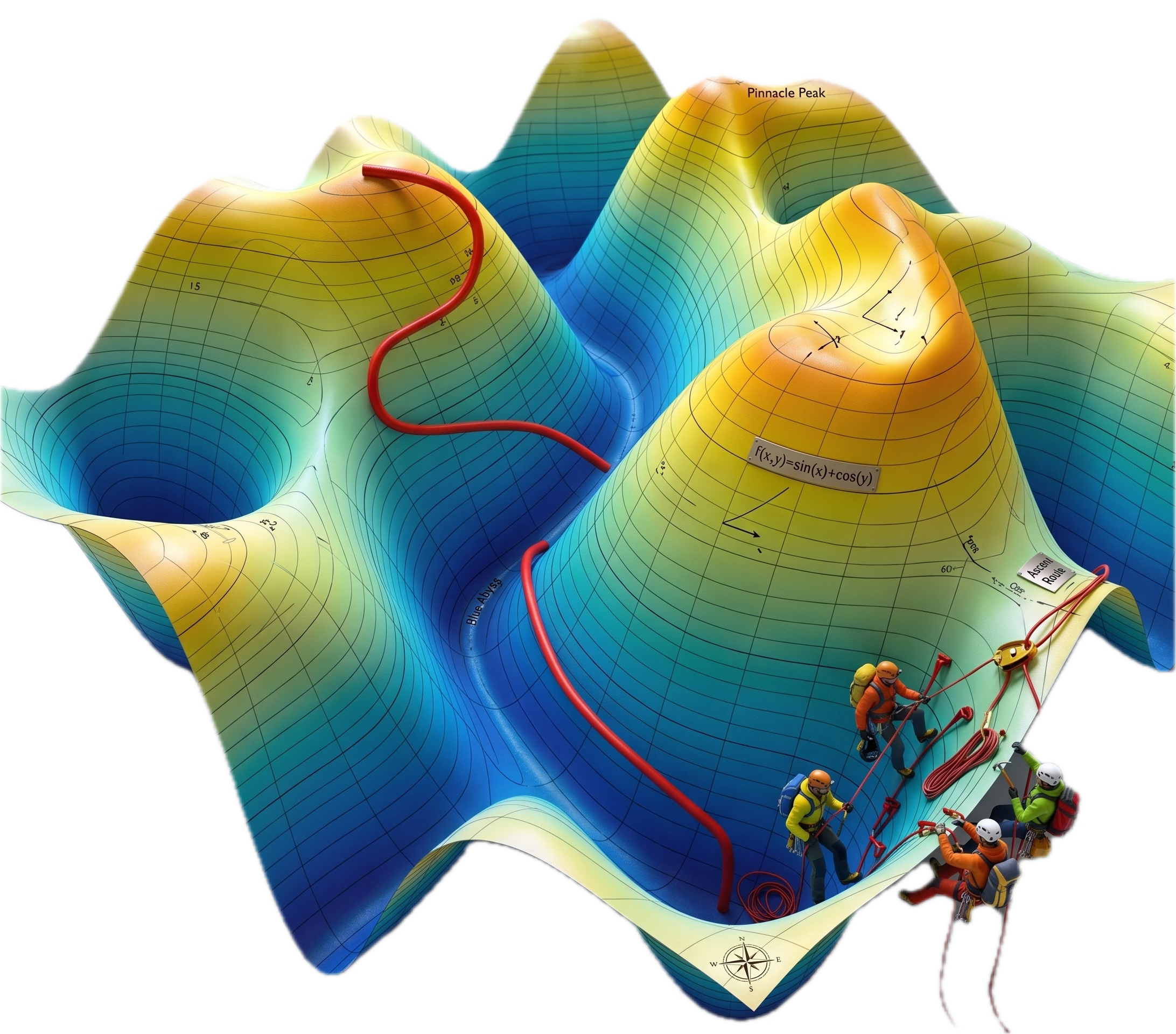
📌 These loss functions are sometimes referred as energy landscape
Quadratic Loss Function
The simplest form of convex function is the ubiquitous quadratic symmetric function. For a two parameters w1, w2 and generic set {w}

Ackley’s Loss Function
The Ackley function is computationally fast regardless of dimensions. It has the following characteristics making it challenging for any optimizer
Non-convexity: Multiple local minima.
Flat regions: The outer edges have very small gradients
Global trend: Despite the noise, the profile has a clear global trend toward the center.
The loss function has 3 components:.
The Exponential Term: Creates the overall shape of global minimum that pulls the optimizer toward the center.
The Cosine Term: Creates the local minima that litter the landscape.
The Constants: These are chosen to ensure the global minimum is exactly at f(0,0) = 0

Rosenbrock’s Loss Function
The Rosenbrock Function is a non-convex function used as a performance test for optimization algorithms. It is famous because the global minimum sits inside a very narrow, parabolic-shaped flat valley.
Because the valley is so narrow and curved, algorithms that use simple gradient descent will often "bounce" back and forth between the walls of the valley (oscillating) rather than moving along the floor toward the minimum.
For a two parameters model the loss function can be samples with the following function.

⚙️ Hands‑on with Python
Environment
Libraries: Python 3.12.5, Numpy 2.3.5, PyTorch 2.7.2
Implementation code: geometriclearning/deeplearning/loss/sgld.py
Evaluation code: geometriclearning/play/sgld_eval_play.py
The source tree is organized as follows: features in python/, unit tests in tests/, and newsletter evaluation code in play/.
To enhance the readability of the algorithm implementations, we have omitted non-essential code elements like error checking, comments, exceptions, validation of class and method arguments, scoping qualifiers, and import statements.
🔎 Implementation
The Stochastic Gradient Langevin Dynamics is implemented in the Python class SGLD which inherits the based class for PyTorch optimizers, torch.optim.Optimizer [ref 6].
The constructor takes two parameters:
params: Model parameters
lr: Learning rate for optimization of the loss function
The step implements the Langevin update formula (6) by adding
Standard stochastic gradient descent component
Normal distributed noise proportional to the square of the learning rate.
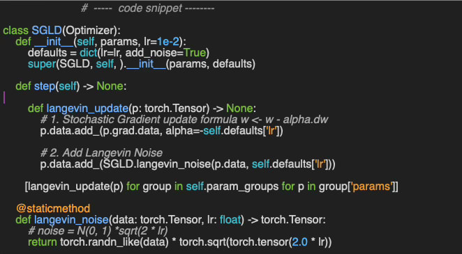
📌 The scale factor for the Gaussian noise in the Langevin component is a function of the learning rate which may depend on the type of application. I used the commonly used square root function.
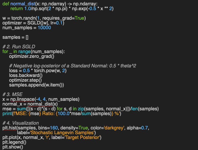
Validation
Ideally, we should be able to unit-test our implementation of the Stochastic Gradient Langevin Dynamics without the need of dataset.
The isotropic Gaussian distribution enables us to compare different optimization methods by selecting a standard distribution P which gradient is equal to its parameter w.
The implementation of the unit test is available on the appendix Appendix: Validation SGLD

📊 Evaluation
Impact of Learning Rate
First, we try to quantify the impact of the learning rate on the trajectory of the minimization of the loss function, taking into account that the amplitude of the noise is proportional to the square root of the learning rate - formula 6.
In this test we use the Ackley function.

As expected the rate of convergence toward the target w1=0, w2=0 increases as the learning rate decreases, which could be counterintuitive for those familiar with SGD behavior.
📌 This test does not tell the whole story; A low learning rate may cause SGLD to converge to a non-global minimum as illustrated below
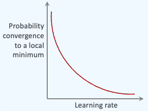
A larger learning rate increases the energy for exploration, while a decaying learning rate allows the system to lock into a stable state (exploitation).
Optimizers Evaluation
The evaluation consist of comparing the trajectory of the minimization of the loss function for 3 optimizers:
SGD
Adam
SGLD
using quadratic and Ackley functions described in the previous section.
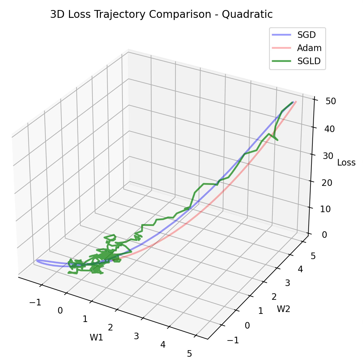
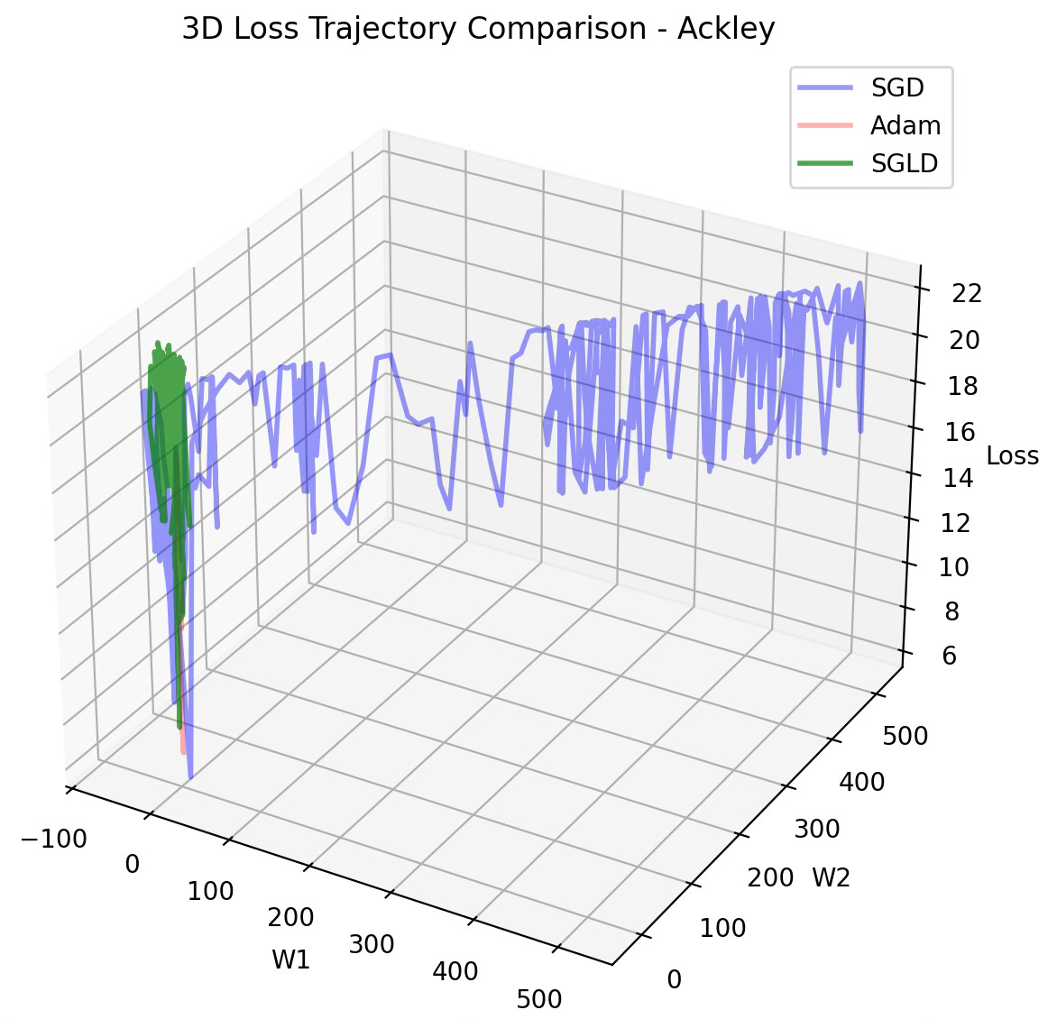
A complex parameters landscape for loss function requires SGD to lower the learning rate to avoid converging to a local minimum, resulting in higher computation cost. The stochastic component of SGLD resolves this issue as illustrated in the previous diagram.
🧠 Key Takeaways 💎
✅ By injecting “controlled jitter” (Gaussian noise) into the update step, SGLD successfully hops out of the shallow local minima that often trap standard gradient-based methods.
✅ Using mathematical “playgrounds” like the Ackley or Rosenbrock functions allows us to isolate and visualize how an optimizer handles complex curvatures before testing on actual data.
✅ PyTorch’s modular design makes SGLD easy to build; you just inherit the Optimizer class and plug your custom logic into the step() method.
✅ Interestingly, SGLD acts as a bridge between worlds: it mirrors the broad exploration of SGD when the learning rate is high and shifts toward the precision of ADAM as the rate cools down.
📘 References
Stochastic Gradient Descent: A Basic Explanation - M. Mishra - Medium, 2023
Gentle Introduction to the Adam Optimization Algorithm for Deep Learning - J. Brownlee - Machine Learning Mastery, 2021
Langevin Dynamics - N. Katz - Towards Data Science, 2021
The promises and pitfalls of Stochastic Gradient Langevin Dynamics - N. Brosse, E. Moulines, A. Durmus, 2018
Bayesian Learning via Stochastic Gradient Langevin Dynamics M. Welling, Y. Whye The, 2011
🛠️ Q & A 💎
1️⃣ What are the two fundamental components that constitute the Stochastic Gradient Descent Langevin update rule?
2️⃣ How does treating the loss function as a potential field facilitate the sampling of the parameter space?
3️⃣ What is the main benefit of SGDL compared to traditional stochastic gradient descent in complex non-convex landscapes?
4️⃣ In what ways does the learning rate drives the equilibrium between gradient-driven convergence and noise-driven exploration?
👉 Answers
🧩 Appendix
🔎 This is the implementation of the evaluation of SGLD using 2 parameter model. It computes the Mean Square Error (MSE) between the weighted computed by the optimizer and the optimal weights computed through the test function.
💬 News & Reviews 💎
This section focuses on news and reviews of papers pertaining to geometric deep learning and its related disciplines.
Paper Review: AI Must Embrace Specialization via Superhuman Adaptable Intelligence - J. Goldfeder, P. Wyder, Y. LeCun, R. Shwartz-Ziv, 2026
This very recent ‘position’ paper is a new perspective on the ever-ending conversation (and speculation) on Artificial General Intelligence (AGI) (without any specific reference to the Joint Embedding Predictive Architecture) . As a starter, we can certainly all agree on the lack of clear and concise definition of AGI.
Instead, Yann LeCun at al introduces the concept of Superhuman Adaptable Intelligence (SAI) with adaptability as its core concept and described through 5, somewhat contrarian, statements:
Human intelligence is factually specialized
Intelligence does not have to be general to be applicable and viable
As mentioned early, the term AGI means anything to anyone
The semantic of intelligence is already well defined
Self-supervised learning and world models
To their credit, the authors provide the reader with alternative/contrarian views (e.g., quotes from Musk, Hassabis on generality of intelligence) and build their arguments upon past studies and reputable papers.
I personally found the following visualization particularly helpful
Organization of the various definition of intelligence using adaptability, generalization and performance through an eye-opening semantic map.
Illustration of overlap of human and AI-tasks
The paper concludes with the theme of adaptability: “SAI is measured by the speed with which it takes an agent to acquire new skills”
Share the next topic you’d like me to tackle.
Patrick Nicolas is a software and data engineering veteran with 30 years of experience in architecture, machine learning, and a focus on geometric learning. He writes and consults on Geometric Deep Learning, drawing on prior roles in both hands-on development and technical leadership. He is the author of Scala for Machine Learning(Packt, ISBN 978-1-78712-238-3) and the newsletter Geometric Learning in Python on LinkedIn.