Riemannian Manifolds: Hands-on with Hypersphere

The hypersphere is the simplest and most visually intuitive geometric structure for applying the knowledge of Riemannian manifolds gained from my previous article, Riemannian Manifolds: 1 Foundation
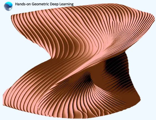
Table of Contents
🎯 Why this Matters
Purpose: Introduction to smooth and Riemannian manifolds as a core concept of Geometric Deep Learning.
Audience: Data scientists and engineers with basic understanding of machine learning. The reader may benefit from prior knowledge in differential geometry.
Value: Understanding fundamental concepts of data manifolds, including metrics, tangent spaces, geodesics, and intrinsic representations, using Python and the Geomstats library.
🎨 Modeling & Design Principles
This references the previous post, which introduces the fundamental components of smooth manifolds, including tangent spaces, geodesics, exponential and logarithm maps, intrinsic and extrinsic geometries, and Lie groups {ref 1].. Riemannian Manifolds: 1 Foundation
I strongly recommend that readers unfamiliar with the fundamental concepts of manifolds, differential geometry, and their importance in Geometric Deep Learning explore the suggested readings in the references [ref 2, 3, 4 & 5].
⚙️ Hands-on with Python
Environment
Libraries: Python 3.11, Geomstats 2.7.2, Scikit-learn 1.4.2
Source code: Github.com/patnicolas/geometriclearning/geometry/manifold
To enhance the readability of the algorithm implementations, we have omitted non-essential code elements like error checking, comments, exceptions, validation of class and method arguments, scoping qualifiers, and import statements.
Geomstats is an open-source, object-oriented library following Scikit-Learn’s API conventions to gain hands-on experience with Geometric Learning. It is described in article Introduction to Geomstats for Geometric Learning
Geomstats Library
The inner workings of the Geomstats library will be the subject of a future post. Here is a quick summary.
Geomstats is a free, open-source Python library designed for conducting machine learning on data situated on nonlinear manifolds, an area known as Geometric Learning. This library offers object-oriented, thoroughly unit-tested features for fundamental manifolds, operations, and learning algorithms, compatible with various execution environments, including NumPy, PyTorch, and TensorFlow [ref 6].
The library is structured into two principal components:
geometry: This part provides an object-oriented framework for crucial concepts in differential geometry, such as exponential and logarithm maps, parallel transport, tangent vectors, geodesics, and Riemannian metrics.
learning: This section includes statistics and machine learning algorithms tailored for manifold data, building upon the scikit-learn framework.
Intrinsic & Extrinsic Geometries
To enhance clarity and simplicity, we've implemented a unique approach that encapsulates the essential elements of a data point on a manifold within a data class.
First we encapsulate the key components of a point on a manifold into a data class ManifoldPoint for convenience with the following attributes:
id A label a point
location A n--dimension Numpy array
tgt_vector An optional tangent vector, defined as a list of float coordinate
geodesic An optional flag to specify if geodesic has to be computed.
intrinsic An optional flag to specify if the coordinates are intrinsic, if True, or extrinsic if False.
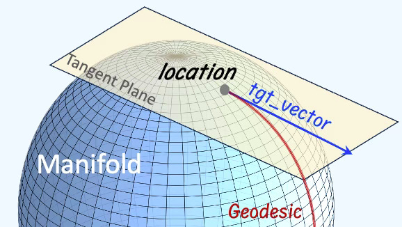
Fig. 1 Illustration of a ManifoldPoint instance
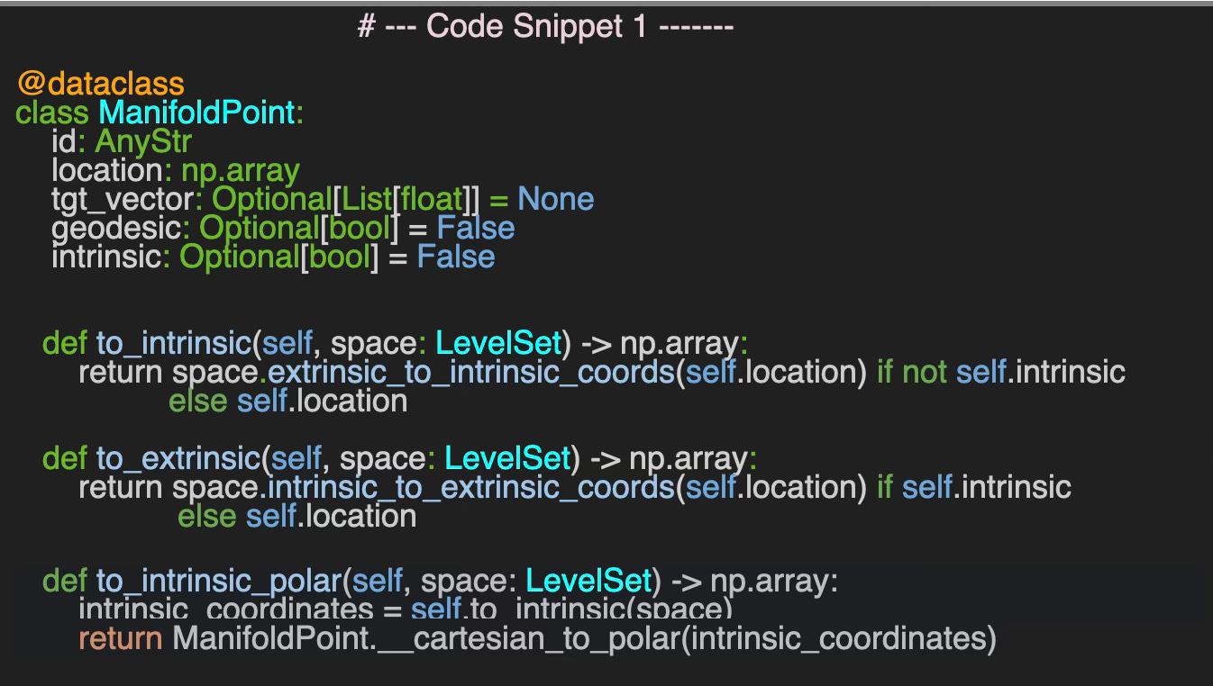
The class ManifoldPoint has 3 methods to define its location given a coordinate system:
to_intrinsic: Convert the current location from extrinsic cartesian coordinates (3 dimension) to intrinsic cartesian coordinates (2 dimension) if the flag intrinsic is False
to_extrinsic: Convert the location from intrinsic cartesian coordinates to extrinsic coordinates if the flag intrinsic is True
to_intrinsic_polar: Convert the current location from extrinsic cartesian coordinates (3 dimension) to intrinsic polar coordinates (2 dimension) if the flag intrinsic is False
This last method relies on the transformation from Cartesian to Polar coordinate on the tangent plane.
The following figure illustrates the transformation from cartesian coordinates (x, y) to polar coordinates (r, theta)
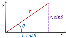
Fig. 2 Visualization of polar coordinates on 2 dimension surface
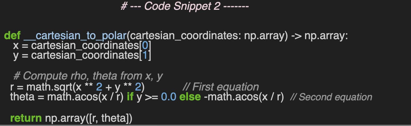
Here are the mathematical equations for the transformation from cartesian to polar coordinates.
The following private static method __cartesian_to_polar , which executes the two formulas, is straightforward.
Hypersphere
Let's build a HypersphereSpace as a Riemannian manifold defined as a spheric 3D manifold space of type Hypersphere and a metric hypersphere_metric of type HypersphereMetric.
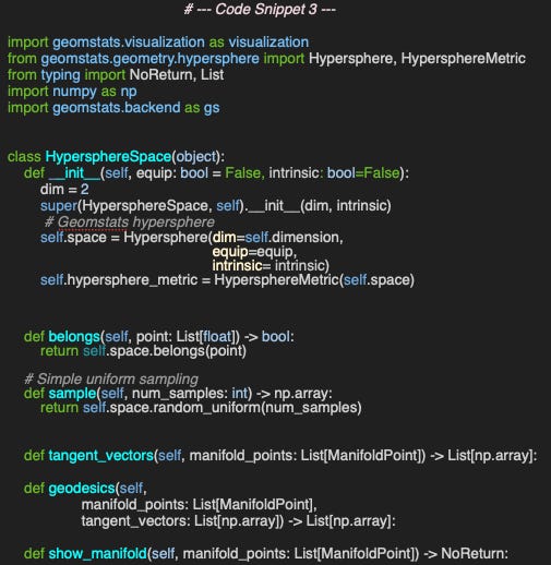
The first two methods to generate and validate data point on the manifold are
belongs to test if a point belongs to the hypersphere
sample to generate points on the hypersphere using a uniform random generator
Tangent Vectors
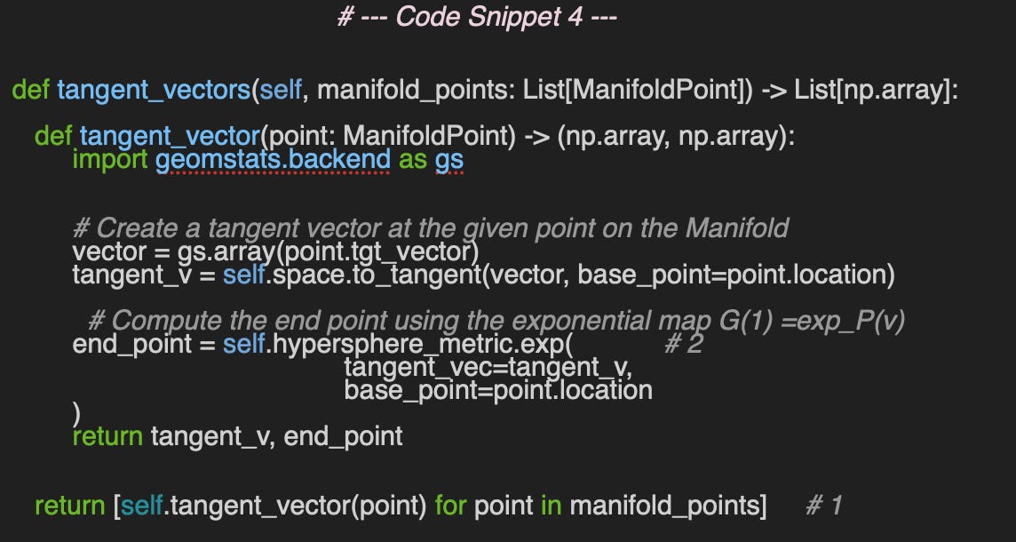
The method tangent_vectors computes the tangent vectors for a set of manifold point defined with their id, location, tgt_vector and geodesic flag. The implementation relies on a simple comprehensive list invoking the nested function tangent_vector (#1). The tangent vectors are computed by projection to the tangent plane using the exponential map associated to the metric hypersphere_metric (#2).
This is the implementation of the formula, described in the previous article [ref 1]
This test consists of generating 3 data points, samples on the hypersphere and construct the manifold points through a comprehensive list with a given vector [0.5, 0.3, 0.5] in the Euclidean space and geodesic disabled.
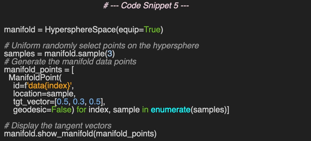
The code for the method show_manifold is described in the Appendix. The execution of the code snippet produces the following plot using Matplotlib.
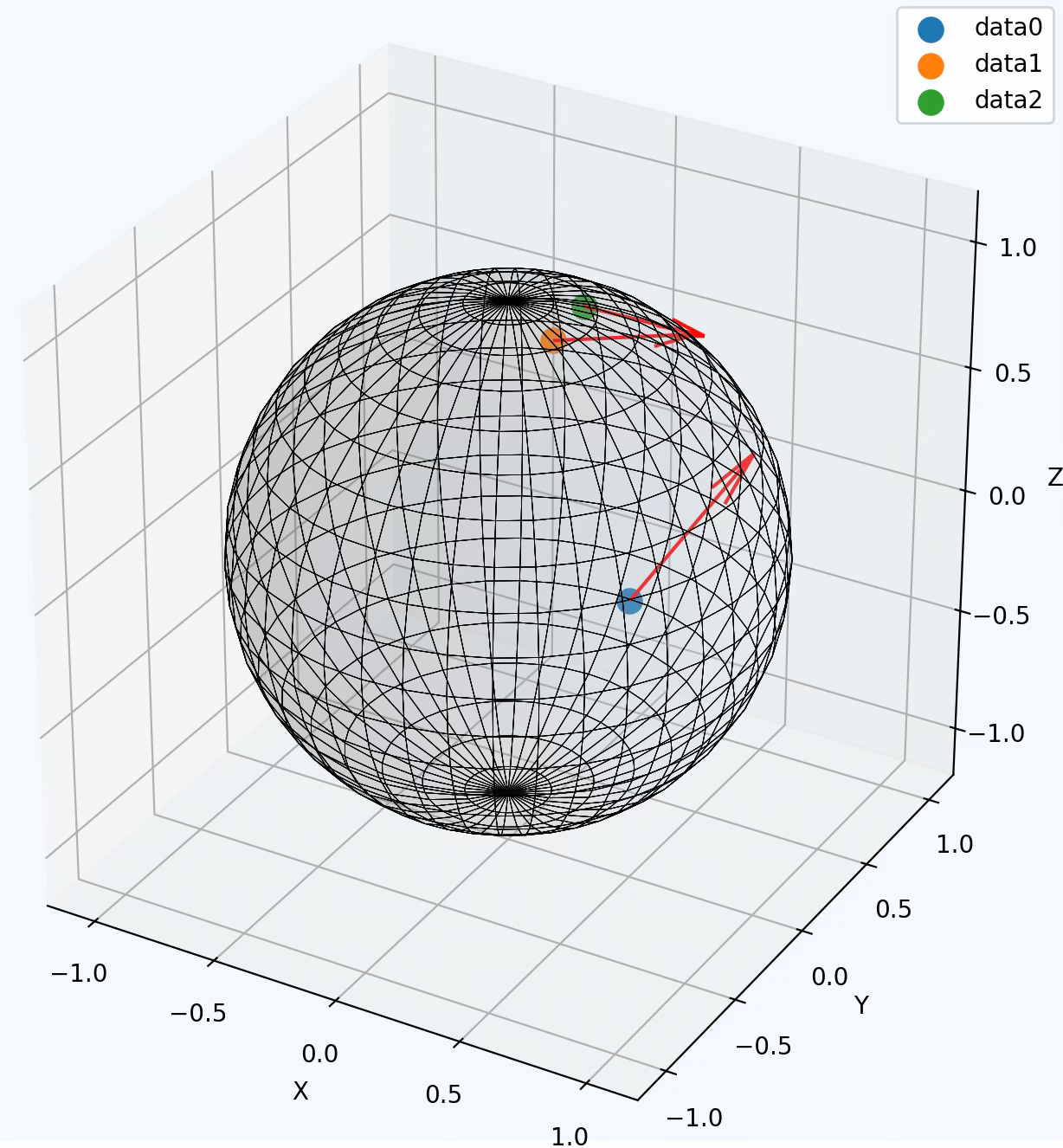
Fig. 3 Visualization of three random data points and their tangent vectors on Hypersphere
Geodesics
The geodesics method calculates the trajectory on the hypersphere for each data point in manifold_points, using the tangent_vectors. Similar to how tangent vectors are computed, the determination of geodesics for a group of manifold points is guided by a Python comprehensive list to invoke the nested function geodesic.
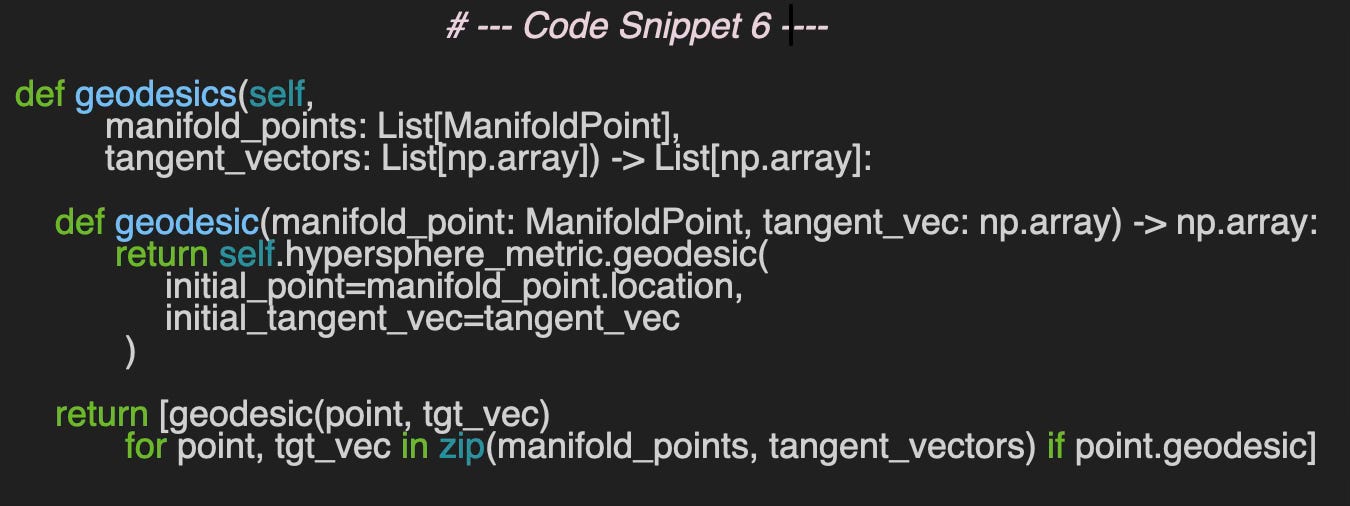
The geodesic is visualized by plotting 40 intermediate infinitesimal exponential maps created by invoking linspace function as described in Appendix.
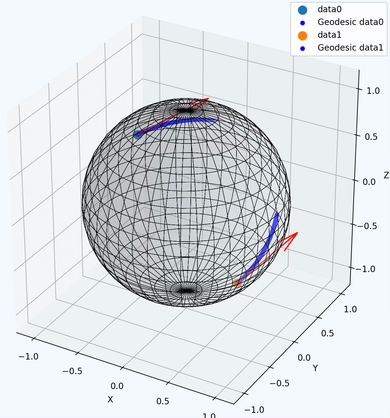
Fig. 4 Visualization of two random data points with tangent vectors and geodesics on Hypersphere
🧠 Takeaways
✅ Geomstats is a free, open-source, object-oriented Python library designed for machine and deep learning on data residing on non-linear manifolds.
✅ The conversion between Cartesian and polar coordinates serves as a clear example of intrinsic vs. extrinsic geometries.
✅ The hypersphere is a 3D manifold that provides an excellent use case for illustrating and visualizing data on manifolds, geodesics, and tangent vectors.
📘 References
Differential Geometric Structures W. Poor - Dover Publications, New York 1981
Introduction to Smooth Manifolds J. Lee - Springer Science+Business media New York 2013
🛠️ Exercises
Q1: What are the two main modules of the Geomstats library? Which module is specifically dedicated to differential geometry?
Q2: Given a point with coordinates (x, y), write a Python function to convert it to polar coordinates (rho, theta).
Q3: When computing and visualizing data points on the hypersphere, should the coordinates be intrinsic?
Q4: What are the two required arguments of the exponential map on the hypersphere, used to compute the endpoint on the manifold?
Q5: What is the relationship between computing an endpoint using the exponential map and computing a geodesic?
👉 Answers
💬 News & Reviews
This section focuses on news and reviews of papers pertaining to geometric deep learning and its related disciplines.
Paper review: Machine Learning Algebraic Geometry for Physics J. Bao, Y-H, He, E Heyes, E Hirst
This paper is a valuable contribution to any discussion or teaching on Information Geometry (refer to the mentioned source).
While some are accustomed to applying laws of Physics, like Partial Differential Equations, to restrict deep learning models in machine learning, the use of machine learning combined with algebraic/differential geometry to process large datasets produced by physics is relatively unusual.
The paper utilizes the Calabi-Yau manifold, derived from the string theory concept of a 10-dimensional spacetime landscape. It examines unsupervised models such as PCA, Topology Data Analysis, Clustering, and then explores neural networks used for data analysis on hypersurfaces. The authors delve into a variety of subjects including projecting to lower-dimensional spaces, Hilbert series, interactions, and equivalences of Branes, as well as cluster mutations.
The study concludes by discussing the optimal transport problem and Kahler geometry in the context of Generative Adversarial Networks.
Reference: Information Geometry: Near Randomness and Near Independence - K. Arwini, C.T.J. Dobson – Springer 2008
Patrick Nicolas has over 25 years of experience in software and data engineering, architecture design and end-to-end deployment and support with extensive knowledge in machine learning.
He has been director of data engineering at Aideo Technologies since 2017 and he is the author of "Scala for Machine Learning", Packt Publishing ISBN 978-1-78712-238-3 and Geometric Learning in Python Newsletter on LinkedIn.
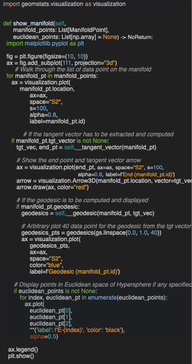
💻 Appendix
The implementation of the method show_manifold is shown for reference. It relies on the Geomstats visualization library. The various components of data points on manifold (location, tangent vector, geodesics) are displayed according to the values of their attributes. Points on 3-dimension Euclidean space are optionally display for reference.