

Riemannian Manifolds: Foundational Concepts
Geometric Deep Learning / Manifolds

Intrigued by the idea of applying differential geometry to machine learning but feel daunted? Beyond theoretical physics, the Riemannian manifolds are essential for understanding motion planning in robotics, object recognition in computer vision and visualization.
Geometric Deep Learning, World Models use complex math to overcome limitations of traditional deep learning. We make that math practical through hands-on tutorials.
Riemannian Manifolds Deep Dive
🏛️ Ricci Tensor Curvature & Flow

👉 Patrick Nicolas is a 30-year software engineering veteran and consultant specializing in Geometric Deep Learning and World Models, author of Scala for Machine Learning, and writer of Geometric Learning in Python.
Why this Matters
Purpose: Introduction to smooth and Riemannian manifolds as a core concept of Geometric Deep Learning.
Audience: Data scientists and engineers with basic understanding of machine learning. The reader may benefit from prior knowledge in differential geometry.
Value: Understanding fundamental concepts of data manifolds, including metrics, tangent spaces, geodesics, and intrinsic representations, using Python and the Geomstats library.
Key Takeaways
The manifold is a fundamental concept in differential geometry, allowing data scientists to model highly non-linear structures.
Manifolds possess a local Euclidean structure known as the tangent space, where linear algebra, tensor computations, calculus, and standard machine learning algorithms remain applicable.
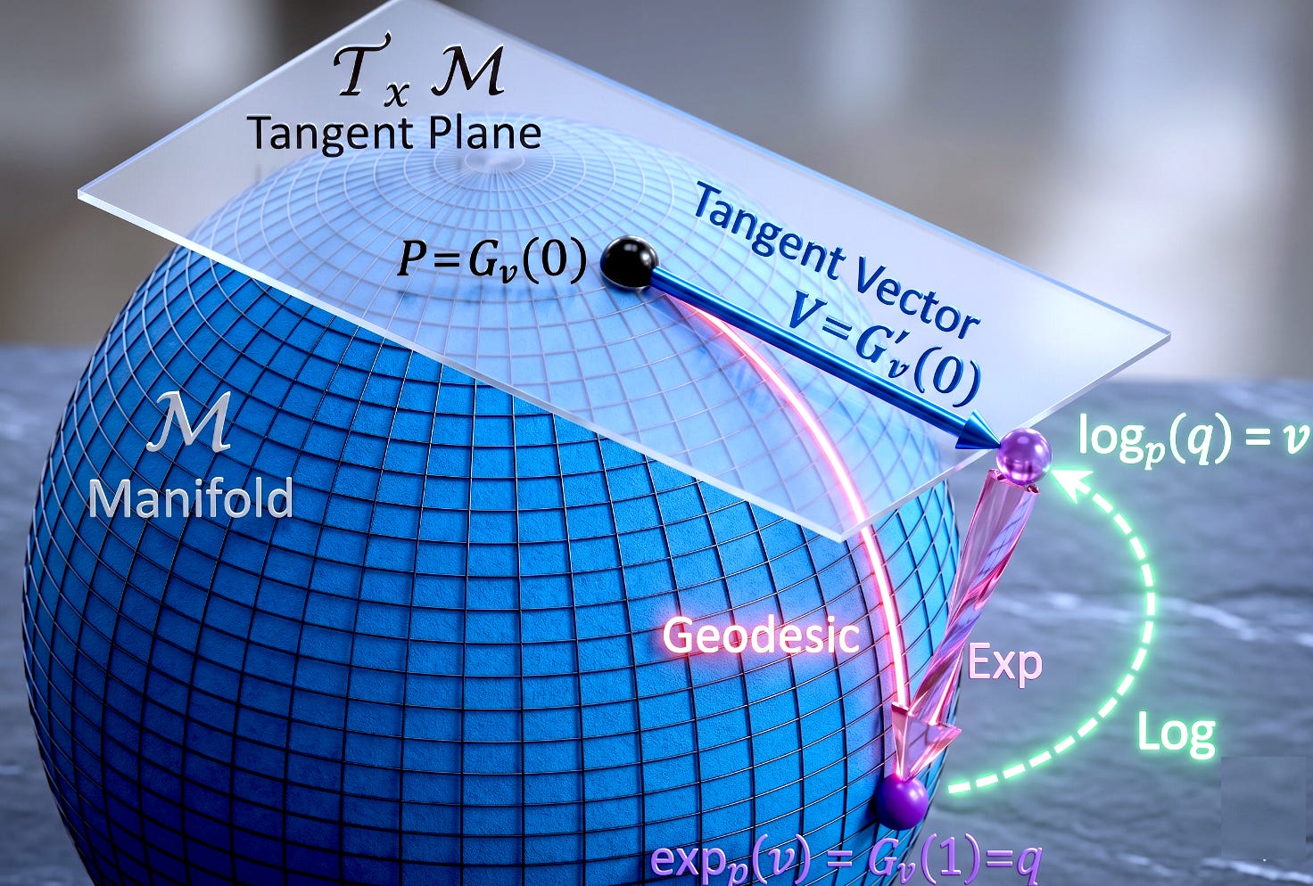
Mapping between the tangent space and the Riemannian manifold is achieved through the exponential map (to the manifold) and the logarithm map (from the manifold).
Data points, vectors, and tensors can be expressed using either intrinsic coordinates relative to the manifold at a specific point or extrinsic coordinates relative to the ambient Euclidean space in which the manifold is embedded.
Riemannian Manifolds Basics
This section covers the essential Basics, while the Deep Dive section delivers advanced concepts, real-world applicability, dedicated Q&A and review.
This is the first part of our introduction to manifolds and their role in Geometric Deep Learning. This post covers the mathematical foundations, with a focus on differential geometry. The second installment will apply these concepts using the hypersphere.
I highly recommend that readers unfamiliar with the fundamental concepts of differential geometry and their significance in Geometric Deep Learning explore Introduction to Geometric Deep Learning
📌 This article focuses on smooth manifolds and continuous differential geometry; however, complex data structures like graphs or simplicial complexes require discrete methods, such as Ollivier-Ricci curvature, Gauss curvature or Euler characteristics treated in different articles [ref 10].
🏛️ Limitation of Euclidean Geometry
⚠️ Real datasets often lie on stratified spaces defines as unions of manifolds with different dimensions). Classical manifold learning theory does not fully address training models on data spread over a heterogeneous set of manifolds,
Geometric Deep Learning addresses the difficulties of limited data, high-dimensional spaces, and the need for independent representations in the development of sophisticated machine learning models, including graph-based and physics-informed neural networks. Data scientists face challenges when building deep learning models that can be addressed by geometric, non-Euclidean representation of data [ref 1].
Here are some of the limitations of relying Euclidean space to build models.
Euclidean space is flat while real-world data distributions lie on highly curved manifolds. Forcing a curved data manifold into a flat Euclidean latent space introduces significant distortion
To embed a hierarchical tree structure into Euclidean space with low distortion would require high dimensional space. This leads to the curse of dimensionality,
The real world is filled with non-trivial global structures: periodic cycles, loops, and closed surfaces. Euclidean spaces can be continuously shrunk to a single point and cannot natively represent topological features such as holes, voids without tearing the data apart.
Euclidean space treats all directions uniformly. It naturally pulls interpolations toward the mean reducing the information from the complex world dynamics.
The primary goal of learning Riemannian geometry is to understand and analyze the properties of curved spaces that cannot be described adequately using Euclidean geometry alone [ref 2].
🏛️ Differential Geometry
Differential geometry is an extensive and intricate area that exceeds what can be covered in a single article or blog post. There are numerous outstanding publications, including books [ref 3, 4, 5, 6], papers [ref 7] and tutorials [ref 8], that provide foundational knowledge in differential geometry and tensor calculus, catering to both beginners and experts
The following highlights the advantages of utilizing differential geometry to tackle the difficulties encountered by researchers in the creation and validation of generative models [ref 3].
Understanding data manifolds: Data in high-dimensional spaces often lie on lower-dimensional manifolds. Differential geometry provides tools to understand the shape and structure of these manifolds, enabling generative models to learn more efficient and accurate representations of data.
Improving latent space interpolation: In generative models, navigating the latent space smoothly is crucial for generating realistic samples. Differential geometry offers methods to interpolate more effectively within these spaces, ensuring smoother transitions and better quality of generated samples.
Optimization on manifolds: The optimization processes used in training generative models can be enhanced by applying differential geometric concepts. This includes optimizing parameters directly on the manifold structure of the data or model, potentially leading to faster convergence and better local minima.
Geometric regularization: Incorporating geometric priors or constraints based on differential geometry can help in regularizing the model, guiding the learning process towards more realistic or physically plausible solutions, and avoiding overfitting.
Advanced sampling techniques: Differential geometry provides sophisticated techniques for sampling from complex distributions (important for both training and generating new data points), improving upon traditional methods by considering the underlying geometric properties of the data space.
Enhanced model interpretability: By leveraging the geometric structure of the data and model, differential geometry can offer new insights into how generative models work and how their outputs relate to the input data, potentially improving interpretability.
Physics-Informed Neural Networks: Projecting physics law and boundary conditions such as set of partial differential equations on a surface manifold improves the optimization of deep learning models.
Innovative architectures: Insights from differential geometry can lead to the development of novel neural network architectures that are inherently more suited to capturing the complexities of data manifolds, leading to more powerful models.
🏛️ Smooth Manifolds
Core Concepts
To refresh your memory, here are some fundamental elements of a manifold:
A manifold is a topological space that, around any given point, closely resembles Euclidean space. Specifically, an n-dimensional manifold is a topological space where each point is part of a neighborhood that is homeomorphic to an open subset of n-dimensional Euclidean space. Examples of manifolds include one-dimensional circles, two-dimensional planes and spheres, and the four-dimensional space-time used in general relativity.
Smooth or Differential manifolds are types of manifolds with a local differential structure, allowing for definitions of vector fields or tensors that create a global differential tangent space.
A Riemannian manifold is a differential manifold that comes with a metric tensor, providing a way to measure distances and angles.
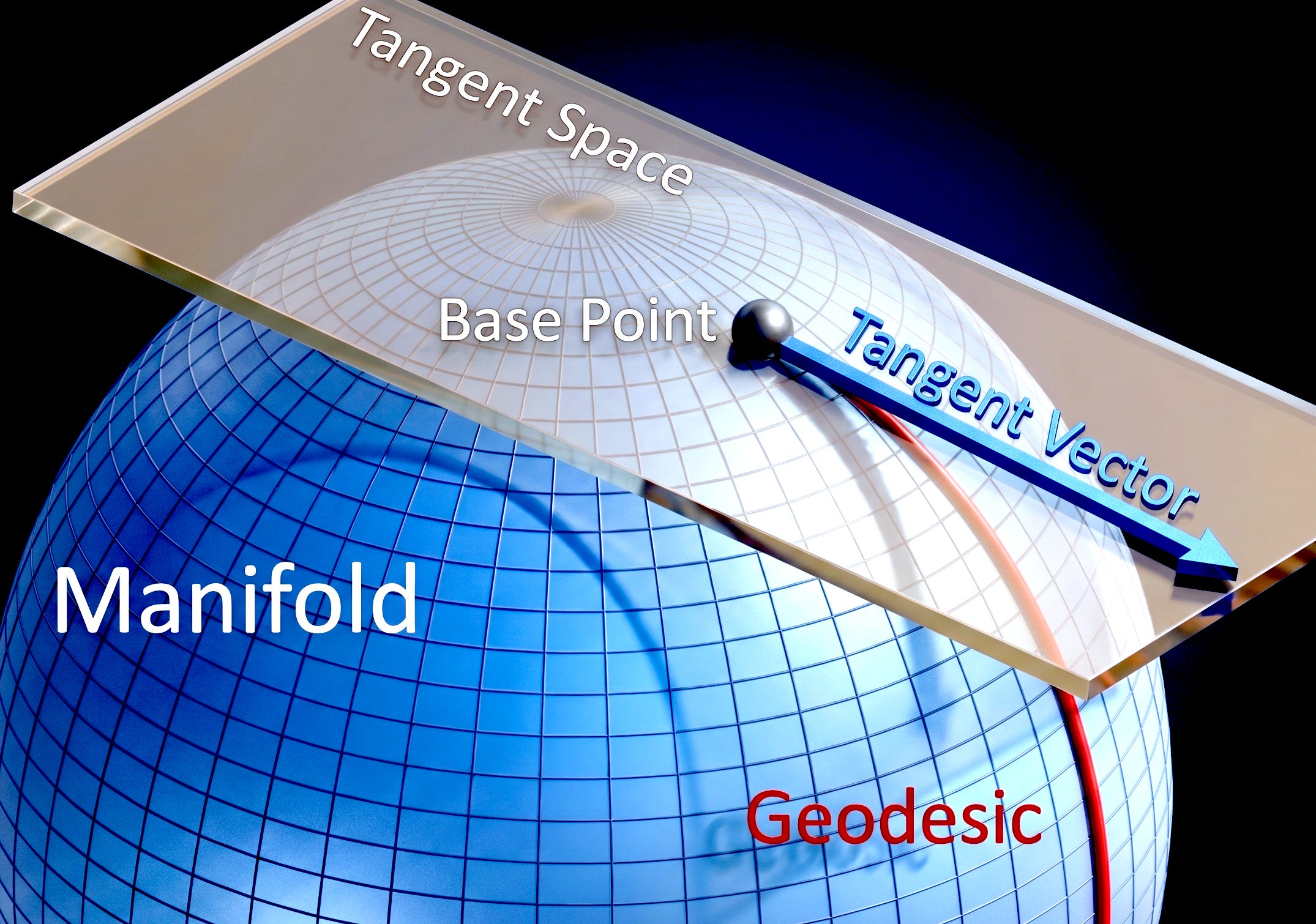
The tangent space at a point on a manifold is the set of tangent vectors at that point, like a line tangent to a circle or a plane tangent to a surface. Tangent vectors can act as directional derivatives, where you can apply specific formulas to characterize these derivatives.
A geodesic is the shortest path (arc) between two points in a Riemannian manifold.
Vector, Tensor Fields & Differential Forms
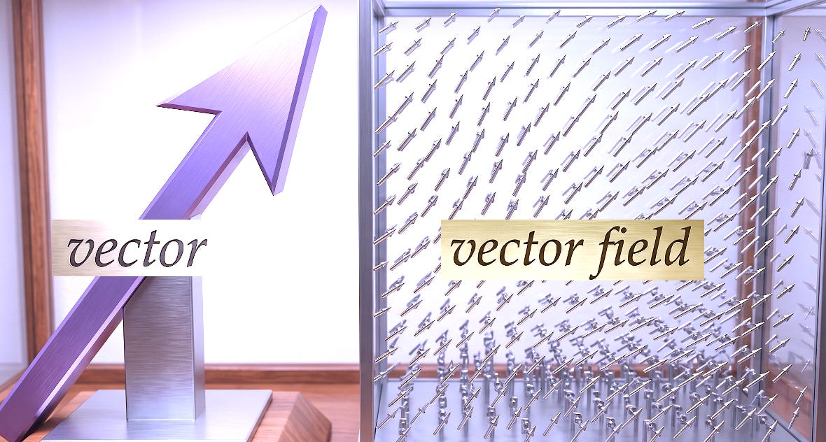
A vector is an arrow pointing through space. A covector is an object that measures vectors moving through space. A covector is a measurement dual to that arrow. While a vector is visualized as an arrow, a covector is best visualized as a set of parallel, evenly spaced hyperplanes(lines in 2D, planes in 3D).
Tensors are multidimensional arrays of numbers that obey specific transformation laws when changing coordinate systems. They track complex, multi-directional relationships.
A vector field assigns a single vector to every point in a space. You can visualize it as an infinite collection of arrows, where each arrow's base sits at a specific point, its direction points where something is moving or pulling, and its length represents intensity.
A tensor field is a generalization of a vector field. Instead of assigning a simple arrow to every point, it assigns a tensor to every point.
📌 Vectors are contravariant as their component values scale inverse to the coordinate system. Covectors are covariant as their components scale with the coordinate system
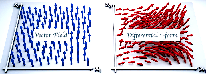
A differential 1-form (a.k.a. covector field) assigns a covector to every point on a space or manifold. Instead of a field of arrows flowing through space, a covector field looks like a topographical contour map.
Intuitively, the directional derivative measures how a function changes as you move in a specific direction. The directional derivative
is large and positive, the function is increasing quickly in that direction.
is zero, the function doesn't change in that direction.
is negative, the function is decreasing in that direction.
From the perspective of the manifold (intrinsic view):
If you move in the direction of the steepest ascent (the gradient direction), the directional derivative is at its maximum.
If you move perpendicular to the gradient, the directional derivative is zero (meaning the function isn't changing in that direction).
If you move in the direction of descent, the directional derivative is negative.

Given a metric g, a covector ω is defined as a linear map
A vector fields v is defined as
A differential 1-form α is defined as
Given a differentiable function f, a vector v in Euclidean space Rn and a point x on manifold, the directional derivative in v direction at x is defined as:
and the tangent vector at the point x is defined as
The gradient can be expressed intrinsically using the Riemannian metric g

Differential k-forms extends the concept of differential 1-form to tensor fields. For instance, a differential 2-form measures a 2-vector fields
Geodesic & Exponential Map
A geodesic is the shortest path between two points in a Riemannian manifold.
An exponential map is a map from a subset of a tangent space of a Riemannian manifold while the logarithm map assign a tangent vector to a point on the manifold as illustrated below.
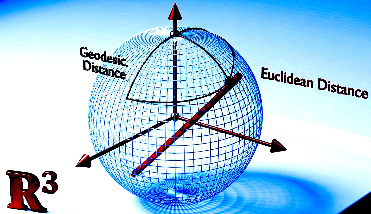
The difference between the geodesic and Euclidean distance is commonly illustrated by flight routes over the globe.

The geodesic is computed through a differential equation:
The geodesic differential equation can be expressed using the Christoffel symbols
Given a Riemannian manifold M with a metric tensor g, the geodesic length L of a continuously differentiable curve f: [a, b] -> M
Given a tangent vector v at a point p on a manifold, there is a unique geodesic Gv and a exponential map exp that satisfy:

Riemannian Metric & Levi-Civita Connection
Riemannian Metric
The Riemannian metric g is an operator that assigns an inner product to the tangent space at every single point on the manifold. The Riemannian Metric is a smoothly varying, positive-definite inner product on each tangent space. I allows the calculation of length, angle and volume associated with vector fields.
Levi-Civita connection
As seen previously, a tangent space at one point of the manifold is ‘tilted’ differently than the tangent space at another point. Therefore, you cannot directly compare vectors from two different tangent spaces because they live in entirely different vector spaces. The Levi-Civita connection solves this issue by providing a consistent rule for directional differentiation and parallel transport. Levi-Civita Connection is a torsion free (symmetric) Riemannian connection.
The Levi-Civita connection imposed two strict conditions:
Metric compatibility: The length and angle between vectors does not change along a path
Torsion-free: The geodesics are the straightest possible paths.
A Killing field is a vector field on a Riemannian or pseudo-Riemannian manifold that preserves the metric.
Christoffel symbols
Christoffel symbols answer the question: How much does the basis vector of coordinate x(I) tilt or stretch into the direction of coordinate x(k) when moving along x(i)?
The Christoffel symbols are computed from metric tensor g expressed in a chosen coordinate system, and its partial derivatives with respect to those coordinates, using the Einstein summation. These symbols account for how your coordinate grid bends, stretches, or twists beneath you as you move across a curved space.
📌 The Christoffel symbols are zeroes in cartesian coordinate in flat (Euclidean) space.
Example: Given line element ds on a 2D sphere of radius r with coordinates θ & ϕ
Given the directional derivative of V along U and V along U, the Levi-Civita connection is expressed as.
A vector field X is a Killing field if the Lie Derivative L of the metric tensor g with respect of X is null
For a Levi-Civita connection, the killing field is expressed as
The formalism for the Christoffel symbols is
Index i: The direction x(i) you are moving along the manifold
index j: The basis vector x(j) you are tracking
index k: The component of the change
The Christoffel Symbol can be expressed, intrinsically using the Riemannian metric.
Keep reading with a 7-day free trial
Subscribe to Hands-on Geometric Deep Learning to keep reading this post and get 7 days of free access to the full post archives.