

Persistent Homology for the Rest of Us
Geometric Deep Learning / Topology

Persistent homology has numerous applications in material science (namomaterial), chemistry, biology (protein folding, drug discovery), computer vision (texture & shape recognition), financial time-series analysis, neural science (neural activity) and above all topological deep learning. It offers an elegant and robust framework for separating structural features from noise, revealing the presence of loops, cycles, and singularities without relying on a metric or coordinate systems.
Geometric Deep Learning, World Models use complex math to overcome limitations of traditional deep learning. We make that math practical through hands-on tutorials.
🏛️ Filtration
⚙️ Evaluation

👉 Patrick Nicolas is a 30-year software engineering veteran and consultant specializing in Geometric Deep Learning and World Models, author of Scala for Machine Learning, and writer of Geometric Learning in Python.
Why this Matters
Purpose: Analyzing the overall geometric structure of data on a low-dimensional smooth manifold is notoriously difficult. Persistent homology simplifies this by providing a reliable way to distinguish real features from background noise—allowing us to detect loops, cycles, and singularities based purely on the data’s underlying distance relationships.
Audience: Data scientists and engineers developing world models, geometric or topological deep network or involved in topological data analysis.
Value: Learn to apply Vietoris-Rips filtration to noisy shaped-data, and create persistence diagrams and persistent barcodes using Scikit-learn TDA
Key Takeaways
Persistent Homology: A tool that maps the overall shape of complex data by identifying and tracking structural features (like holes or cavities) at different levels of detail.
Filtration: The process of expanding spheres around data points to build interconnected shapes, noting exactly when new structural features form and when they fill in.
Birth-Death Diagrams: A chart mapping the lifespan of these features, acting as a distinct geometric signature for the dataset.
Persistence Barcodes: A barcode-like chart that illustrates how long each shape feature survives as the scale changes during filtration.
Python Libraries: Scikit-learn TDA along with Ripser library provides a unified interface to specialized Python libraries for persistent homology, making it one of the most convenient tools for generating and manipulating persistence diagrams and persistent barcodes.
Persistent Homology Basics
🏛️ Topological Data Analysis
Many challenges in data analysis echo two fundamental integration problems:
How to recover high-dimensional structure from low-dimensional representations
How to assemble discrete samples into a coherent global form
Topological Data Analysis (TDA) is a methodology that applies concepts from algebraic topology and computational geometry to analyze and extract meaningful patterns from complex datasets. It provides a geometric and topological perspective to study the shape and structure of data [ref 1]. TDA seeks to develop rigorous mathematical, statistical, and algorithmic techniques to infer, analyze, and leverage the intricate topological and geometric structures underlying data, often represented as point clouds in Euclidean or more general metric spaces.
The most common topological domains [ref 2, 3] are
Simplicial Complexes
Cellular Complexes
Hypergraphs
Combinatorial Complexes
Some of the most common concepts used in TDA are:
Persistent homology captures the topological structure of data across different spatial resolutions. Features that remain stable over many scales are interpreted as genuine properties of the space, while short-lived ones are viewed as noise or artifacts.
A chain complex is the study of spaces and shapes in algebraic topology, consisting of a sequence of mathematical objects connected by homomorphisms. Chain complexes are structured so that the composition of any two consecutive maps is zero.
While chain complexes move downward in dimension in the sequence of objects, the cochain complexes, associated with cohomology moves upward in dimension.
A Cohomology from a cochain complex gives algebraic invariants of a space. Compared to homology, cohomology often carries additional structure.
Filtrations of a space across scales give rise to persistent homology, summarizing the birth and death of features; distances between summaries are stable under small perturbations.
Homotopy theory is a branch of algebraic topology that studies the properties of spaces that are preserved under continuous deformations, called homotopies. It helps in distinguishing spaces that are topologically the same from those that are not and offers tools for working with complex spaces in mathematics and applied sciences
🏛️ Persistent Homology
Persistent homology is the process of capturing the global geometric and topological structure of complex data and identifying and tracking features [ref 4, 5, 6] such as loops, cycles, and voids across multiple scales, as illustrated below:
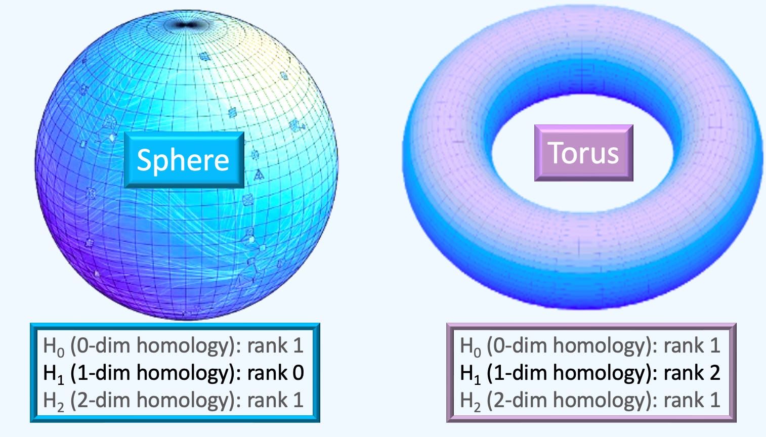
📌 The rank of a homology class Hn is directly associated with the Betti number.
Persistent homology can be summarized as a three-step procedure as follows:
Filtration: Generate a nested sequence of simplicial complexes derived from the data. Through filtration, Persistent Homology tracks the emergence and disappearance of topological features across multiple scales, revealing structural properties of the data that traditional methods often miss.
Persistence diagrams: Record the evolution of topological features across this sequence.
Machine learning integration: Transform the persistence diagrams into vectors for efficient use in ML models.
🏛️ Filtration
The filtration method the most commonly used in Topological Data Analysis is the Vietoris-Rips filtration that can arbitrary be broken down into 3 steps
Growing Spheres: We place a ball of radius ε around each point in space (point cloud).
Building Complexes: We increase ε 0 → infinity, to expand these balls. When two balls intersect, a line segment (1-simplex) connects them. When three intersect, a triangle (2-simplex) forms, creating a simplicial complex.
Birth and Death: The topological features slowly appear and eventually get filled in.
Birth: The radius ε at which a specific topological hole first appears.
Death: The radius ε at which that same hole is filled in or merges into a larger component.
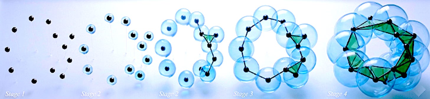
Fig. 2 Visualization of a Vietoris-Rips filtration for 10-point cloud
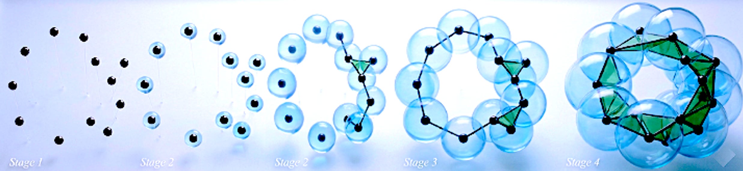
The Čech Filtration is a variant of the Vietoris-Rips filtration. The key difference is adding higher-dimensional simplex only when all the respective balls mutually intersect. This method is more accurate but requires greater computation resources.’

A chain complex C is a sequence of R modules (e.g. vector spaces) and linear maps ∂ called boundary operators, such as
A cochain complex C is a sequence of R modules (e.g. vector spaces) and linear maps d called coboundary operators, such as
A filtration is defined as a sequence of topological Xi spaces of increasing size
The dimension of the homology group is defined as
k=0: Connected components
k=1: Loops
k=2: Cavities
…
The k-th homology groups Hk for each of the topological space Xi and its induced linear map i associated to the inclusion.

📌 A chain complex moves downward in dimension while a cochain moves upward in dimension
I select a simple 6-point cloud evenly distributed in a circle to illustrate the steps of filtration.
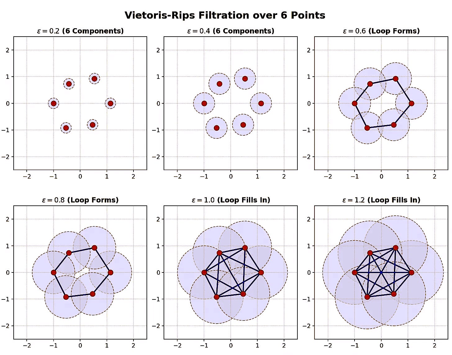
Filtration stages:
A ball of diameter ε is assigned to each of the original 6 components (or points).
Although the size of the ball increases the components are still independent
As ε increases, the simplices overlap around a circle to create a loop form as a new complex
At this stage, ε = 0.8, the only edges created are between consecutive components of the loop simplex
The filtration discovers new edges between components across the loop for ε = 1.0
The filtration process identifies all possible edges (15), as ε increases toward infinity
📌 The maximum number of edges of an undirected graph with n nodes are
📚 TDA Libraries
Scikit-learn TDA
The scikit-learn TDA package generally refers to the ecosystem of Topological Data Analysis tools that follow the scikit-learn API, most notably the packages from the scikit-TDA organization [ref 7].
Practically, scikit-TDA is a collection of Python libraries that bring Topological Data Analysis techniques into the scikit-learn workflow such as:
Persistent homology & persistence diagrams
Vietoris–Rips complexes
Topological feature vectors
Machine-learning models leveraging topological domains
Scikit-learn TDA leverages two 3rd party packages
Ripser for fast persistent homology computation
Persim for creating and visualizing persistence diagrams
Installation:
pip install scikit-tdaRipser
Ripser.py is a lean persistent homology package for Python built upon the fast C++ Ripser engine [ref 8]. It supports:
Computing persistence homology & cohomology
Handling both sparse and dense data sets
Approximating sparse filtration
Visualizing persistence diagrams
Computing lowerstar filtrations on images
Computing representative cochains.
Installation:
pip install Cython
pip install Ripser
🔓 The rest of this deep dive is exclusive to paid subscribers. By upgrading, you unlock this full article along with a comprehensive archive of engineering articles, paper review, concept breakdowns, code walkthrough, GitHub repository & Q&A
Keep reading with a 7-day free trial
Subscribe to Hands-on Geometric Deep Learning to keep reading this post and get 7 days of free access to the full post archives.