Hands-on Principal Geodesic Analysis

Jan 25, 2025

Principal Component Analysis (PCA) is essential for dimensionality and noise reduction, feature extraction, and anomaly detection. However, its effectiveness is limited by the strong assumption of linearity.

Principal Geodesic Analysis (PGA) addresses this limitation by extending PCA to handle non-linear data that lies on a lower-dimensional manifold.

Why this Matters

Purpose: Understand and address the limitation of Principal Component Analysis in non-Euclidean data sets.

Audience: Data scientists and engineers with basic understanding of machine learning and linear models. The reader may benefit from prior knowledge in differential geometry.

Value: Learn to implement principal geodesic analysis as extension of principal components analysis on a manifolds tangent space.

Modeling & Design Principles

Overview

As a reminder, the primary goal of learning Riemannian geometry is to understand and analyze the properties of curved spaces that cannot be described adequately using Euclidean geometry alone.

This article revisits the widely used unsupervised learning technique, Principal Component Analysis (PCA), and its counterpart in non-Euclidean space, Principal Geodesic Analysis (PGA).

The content of this article is as follows:

Brief recap of the Principal Component Analysis
Overview of key components of differential geometry
Introduction to PCA on tangent space using the logarithmic map
Implementation in Python using the Geomstats library.

Principal Component Analysis

Principal Component Analysis (PCA) is a technique for reducing the dimensionality of a large dataset, simplifying it into a smaller set of components while preserving important patterns and trends. The goal is to reduce the number of variables of a data set, while preserving as much information as possible. For a n-dimensional data, PCA tries to put maximum possible information in the first component c0, then maximum remaining information in the second c1 and so on.

Finally, we select the p << n top first components such as:

\(\left \{ c_{i} :\ \ \sum_{i=1}^{p} c_{i} < T \ and \ \ c_{1} \geqslant c_{2} .... \geqslant c_{p} \right \}\)

The principal components are actually the eigenvectors of the covariance matrix.

The first thing to understand about eigenvectors and eigenvalues is that they always appear in pairs, with each eigenvector corresponding to an eigenvalue. Additionally, the number of these pairs matches the number of dimensions in the data.

For instance, in a 3-dimension space, the eigenvalues are extracted from the following 3x3 symmetric covariance matrix:

\(\begin{bmatrix} cov(x, x)) & cov(x,y) & cov(x, z)\\ cov(x, y) & cov(y,y) & cov(y,z) \\ cov(x, z) & cov(y, z) & cov(z, z) \end{bmatrix}\)

as cov(x, y) = cov(y, x).

The eigenvectors of the Covariance matrix (principal components) are the directions of the axes where there is the most variance (most information).

Assuming n normalized data points xi, the first principal component (with most significant eigenvalue) is defined as:

\(P_{1}= arg\max_{||p||=1} \sum_{i=1}^{n} \left ( p.x_{i} \right )^{2} \ \ \ (1)\)

where '.' is the dot product.

Differential geometry

Extending principal components to differentiable manifolds requires basic knowledge of differential and Riemann geometry introduced in following articles [ref 2, 3, 4].

Smooth Manifold

A smooth (or differentiable) manifold is a topological manifold equipped with a globally defined differential structure. Locally, any topological manifold can be endowed with a differential structure by applying the homeomorphisms from its atlas and the standard differential structure of a vector space.

Tangent Space

At every point P on a differentiable manifold, one can associate a tangent space, which is a real vector space that intuitively encompasses all the possible directions in which one can move tangentially through P. The elements within this tangent space at P are referred to as the tangent vectors, tgt_vector at P.

This concept generalizes the idea of a vector originating from a specific point in Euclidean space. For a connected manifold, the dimension of the tangent space at any point is identical to the dimension of the manifold itself.

Geodesics

Geodesics are curves on a surface that only turn as necessary to remain on the surface, without deviating sideways. They generalize the concept of a "straight line" from a plane to a surface, representing the shortest path between two points on that surface.

Mathematically, a curve c(t) on a surface S is a geodesic if at each point c(t), the acceleration is zero or parallel to the normal vector:

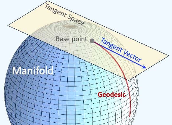
\(\frac{d^{2}}{dt^{2}}c(t) = 0 \ \ or \ \ \frac{d^{2}}{dt^{2}}c(t).\vec{n}=\frac{d^{2}}{dt^{2}}c(t)\)

Fig. 1 Illustration of a tangent vector and geodesic on a sphere

Logarithmic Map

Given two points P and Q on a manifold, the vector on the tangent space v from P to Q is defined as:

\(\left \| log_{P}(Q) \right \| = \left \| v \right \|\)

Tangent PCA

On a manifold, tangent spaces (or plane) are local euclidean space for which PCA can be computed. The purpose of Principal Geodesic Analysis is to project the principal components on the geodesic using the logarithmic map (inverse exponential map).

Given a mean m of n data points x[i] on a manifold with a set of geodesics at m, geod, the first principal component on geodesics is defined as:

\(\begin{matrix} P_{1}=arg\max_{\left \| v \right \| = 1}\sum_{i=1}^{n}\left \langle v.log_{m}\pi _{geod}(x_{i}) \right \rangle^{2} \\ \pi_{geod}(x_{i}) = arg\max_{g \in geod} \left \| log_{m}(x_{i})-log_{m}(g) \right \|^2 \end{matrix}\)

Fig. 2 Illustration of a tangent vector and geodesic on a sphere

Hands-on with Python

Environment

Libraries: Python 3.10.10, Geomstats 2.7.0, Scikit-learn 1.4.2
Source code: Available at GitHub.com/patnicolas/Data_Exploration/manifolds
This article assumes that the reader is somewhat familiar with differential and tensor calculus [ref 1]. Please refer to our articles related to geometric learning [ref 2, 3, 4].
To enhance the readability of the algorithm implementations, we have omitted non-essential code elements like error checking, comments, exceptions, validation of class and method arguments, scoping qualifiers, and import statements.
Geomstats is an open-source, object-oriented library following Scikit-Learn’s API conventions to gain hands-on experience with Geometric Learning. It is described in article Introduction to Geomstats for Geometric Learning

Implementation

For the sake of simplicity, we illustrate the concept of applying PCA on manifold geodesics using a simple manifold, Hypersphere.

To enhance clarity and simplicity, we've implemented a unique approach that encapsulates the essential elements of a data point on a manifold within a data class.

An hypersphere S of dimension d, embedded in an Euclidean space d+1 is defined as:

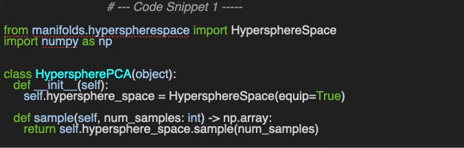
\(S^{d}=\left \{ x\in \mathbb{R}^{d+1} \ | \ \left \| x \right \| = 1\right \}\)

Design

Let's encapsulate the evaluation of principal geodesics analysis in a class HyperspherePCA. We leverage the class HyperphereSpace in Geomstats library [ref 7] its implementation of random generation of data points on the sphere.

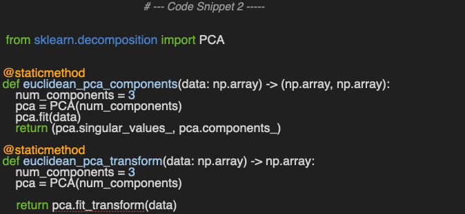
PCA

First let's implement the traditional PCA algorithm for 3 dimension (features) data set using scikit-learn library with two methods:

euclidean_pca_components to extract the 3 eigenvectors along the 3 eigenvalues
euclidean_pca_transform to project the evaluation data onto 3 directions defined by the eigenvectors.

Let’s compute the principal components on 256 random 3D data points on the hypersphere.

Principal components: 
[[ 0.631  -0.775  -0.021]
 [ 0.682   0.541   0.490]
 [ 0.368.  0.324 -0.871 ]]

Eigen values: [9.847 9.018 8.658]

Important note: The 3 eigenvalues are similar because the input data is random.

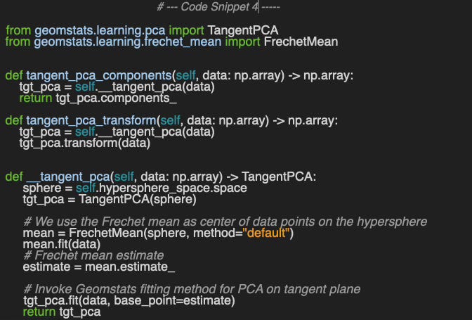
Tangent PCA on Hypersphere

The private method __tangent_pca computes principal components on the tangent plane using the logarithmic map. As detailed in the previous section, this implementation employs the Frechet mean as the base point on the manifold, which is the argument of the Geomstats method fit.

The method tangent_pca_components extracts the principal components computed using the logarithmic map. Finally the method tangent_pca_transform projects input data along the 3 principal components, similarly to its Euclidean counterpart, euclidean_pca_transform.

We evaluate the principal geodesic components on hypersphere using the same 256 points randomly generated on the hypersphere and compared with the components on the Euclidean space.

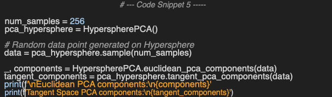
Euclidean PCA components:
[[ 0.631  -0.775 -0.021]
 [ 0.682   0.541   0.490]
 [ 0.368   0.324  -0.871 ]]

Tangent Space PCA components:
[[  0.820  -0.458  0.342]
 [  0.458.  0.167 -0.872]
 [-0.342  -0.872 -0.347]]

Takeaways

PCA's assumption of linearity is inadequate for dense data distributed on a low-dimensional manifold.
Principal Geodesic Analysis (PGA) addresses this limitation by calculating eigenvalues and eigenvectors in the tangent space, using the logarithm map to project data points.
PGA demonstrates superior performance compared to PCA for data points located on a hypersphere.
Geomstats simplifies the transition from PCA in Euclidean space to manifold-based analysis.

References

Exercises

Q1: How does Principal Geodesic Analysis overcome the limitations of Principal Component Analysis?
Q2: What is the purpose of computing the eigenvectors of the covariance matrix?
Q3: Principal components are computed in the locally Euclidean tangent space using:
- Exponential map
- Projection along a geodesic
- Logarithmic map
Q4: How can you extract the singular values and components of PCA using the Scikit-learn library?
Q5: What would be the Euclidean PCA matrix and the Tangent Space PCA matrix when set to 64? 1024?

Exercises Answers

News and Reviews

This section focuses on news and reviews of papers pertaining to geometric deep learning and its related disciplines.

Paper review: Machine Learning & Algebraic Geometry V. Shahverdi 2023

This concise presentation synthesizes and summarizes various research findings at the crossroads of machine learning and algebraic geometry. The author begins by reviewing essential aspects of machine learning, including Kernel methods, feedforward neural networks, and the universal approximation theorem.

Algebraic geometry's application to machine learning

The paper explores how activation functions correlate with the mathematical structure involved in minimizing the loss function under three scenarios:

Linear Neural Networks
Neural Networks employing polynomial approximations for activation.
Networks utilizing ReLU activation.

It defines the space of neural network weights as a low-dimensional manifold, where the loss function's minimization occurs across the weights on this manifold.

Applying machine learning to algebraic geometry

The goal is to comprehend the topology of hypersurfaces using machine learning techniques. Here, a neural network delineates the boundary decision among regions or chambers within hypersurfaces.

Note: The reader would benefit from basic knowledge in algebraic topology and geometry

Patrick Nicolas has over 25 years of experience in software and data engineering, architecture design and end-to-end deployment and support with extensive knowledge in machine learning.
He has been director of data engineering at Aideo Technologies since 2017 and he is the author of "Scala for Machine Learning", Packt Publishing ISBN 978-1-78712-238-3 and Geometric Learning in Python Newsletter on LinkedIn.