Fractal Dimension for Configuring Convolutional Networks

Geometric Deep Learning / Geometry

Challenged by the configuration of Convolutional Neural Networks for complex images?

Incorporating fractal dimension analysis offers a promising strategy. By quantifying structural complexity, this method aids in rationally configuring essential parameters such as kernel size, padding, and pooling.

Geometric Deep Learning, World Models use complex math to overcome limitations of traditional deep learning. We make that math accessible through hands-on tutorials.

---

1. Why this Matters

2. Key Takeaways

3. Fractal Complexity Basics

   Why Fractal Dimension

   What is a Dimension After All

   🏛️ Fractal Dimension

   🏛️ Box Counting Method

   🏛️ Log-log Regression

4. Fractal Complexity Deep Dive

   🏛️ Reference Shapes

   • Line

   • Solid Rectangle

   • Koch Curve

   Python Environment

   Fractal Dimension Pipeline

   ⚙️ Setup

   ⚙️ Image Processing

   ⚙️ Box Counting Implementation

   ⚙️ Evaluation

5. References

6. Q & A

7. Appendix

   ⚙️ Fast Box Counting

   ⚙️ Koch Curve Generation

8. Paper Review

Why this matters

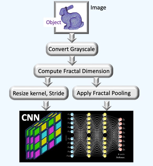
Purpose: Configuring the parameters of a 2D convolutional neural network (CNN), such as kernel size and padding, can be challenging because it largely depends on the complexity of an image or its specific sections. Fractals help quantify the complexity of important features and boundaries within an image and ultimately guide the data scientist in optimizing his/her model.

Audience: Data scientists looking for guidelines to estimate the architectural parameters of a 2D CNN.

Value: Learn basic concept and implementation of the computation of the fractal dimension using the box counting method.

Key Takeaways

• Fractal dimension calculations guide tuning of CNN parameters like kernel size, stride, and pooling.

• The box-counting algorithm estimates the complexity of objects within an image.

• An image pre-processing pipelines removes background artifacts to yield precise fractal dimension measurements.

• The Koch curve is commonly used to validate fractal dimension implementation

Fractals Complexity Basics

I apply fractal dimension computation to the parameterization of convolutional neural networks, though the approach is equally applicable to other deep learning models."

Why Fractal Dimension?

Fractal dimension quantifies the ‘geometric complexity’ of an object or image. Therefore it is useful in configuring parameters and architecture of convolutional networks (CNNs). It bridges the gap between spatial data complexity and model parameterization.

• Configuring receptive fields. A receptive field grows in accordance with the spatial information scaling of the data. For instance, large kernel and stride would accommodate sparse geometrical features to avoid redundancy. Likewise, complex object such as medical imaging or geographic coastlines, need smaller, denser kernels with overlapping (small) strides.

• Fractal Pooling; Max pooling ensures translation invariance by stripping out spatial layout information that may cause the CNN to underperform. A fractal pooling module captures the actual spatial distribution of features - known as Lipschitz invariance.

Fig. 1 Logic for the application of the fractal dimension to the configuration of a Convolutional Neural Network

Lipschitz invariance is the property of a function or transformation to preserve relative distance between data points tup to a bounded scaling factor.

Given 2 metric space (X, d_X) and (Y, d_Y) and a map f: X → Y

\(\exists L\in \mathrm{R}, \ \ \forall x_{1},x_{2} \ \ d_{Y}\left( f(x_{1}), f(x_{2}) \right) \le d_{X}(x_{1}, x_{2})\)

The topology of the space is preserved under deformation if

\(\exists L_{1}, L_{2}\in \mathrm{R}, \ \ \forall x_{1},x_{2} \ \ \ \frac{1}{L_{1}}d_{X}(x_{1}, x_{2}) \le d_{Y}(f(x_{1}), f(x_{2})) \le L_{2}\ d_{X}(x_{1}, x_{2})\)

---

⚠️ How to update a CNN’s configuration using the fractal dimension of embedded objects lies outside the scope of this article and will be covered in a future piece.

---

What is a dimension after all?

Here are 3 definitions of dimension

• Dimension in Euclidean space (line:1, plane: 2, Sphere: 3, ..)

• Number of variables in a dynamic system or features in a model

• Hausdorff dimension: Given an object in a D-dimensional Euclidean space, the measure increases by N=r^D each time its spatial dimension decreases by 1/r

Fig. 2 Illustration of the Hausdorff dimension.

---

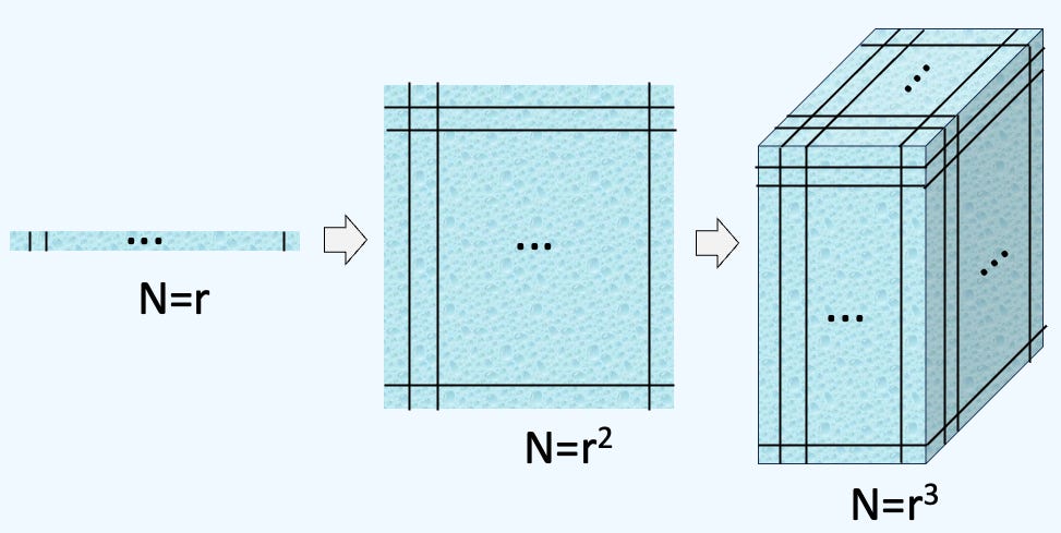
📌 The Hausdorff dimension is not restricted to integers, It can be a floating point values as with fractals.

---

Fractal Dimension

A fractal dimension is a measure used to describe the complexity of fractal patterns or sets by quantifying the ratio of change in detail relative to the change in scale [ref 1].

Initially, fractal dimensions were used to characterize intricate geometric forms where detailed patterns were more significant than the overall shape. For ordinary geometric shapes, the fractal dimension theoretically matches the familiar Euclidean or topological dimension.

However, the fractal dimension can take non-integer values. If a set’s fractal dimension exceeds its topological dimension, it is considered to exhibit fractal geometry [ref 2].

There are many approaches to compute the fractal dimension [ref 1] of an image or a 3D object among them:

• Variation method

• Structure function method

• Root mean square method

• R/S analysis method

• Box counting method

Box Counting Method

The box counting method is similar to the perimeter measuring technique we applied to coastlines. However, instead of measuring length, we overlay the image with a grid and count how many squares in the grid cover any part of the image. We then repeat this process with progressively finer grids, each with smaller squares. By continually reducing the grid size, we capture the pattern's structure with greater precision.

---

📌 The box counting method is also known as the Minkowski–Bouligand dimension.

.

Given the number of boxes of side length ε, N(ε) the box count dimension is computed as

\( D_{box}=-\lim_{\epsilon \to 0} \frac{log(N(\epsilon))}{log(\epsilon)}\)

The limit can be approximated with a Log Power-Law formula

\(Log (N(\epsilon))= -D_{box}.log (\epsilon) + \xi\)

The limit superior and inferior limits are used If the above limit does not exist. Computing the limit can be intractable as we cannot take the limit to absolute zero in a discrete digital grid.

Log-log Regression

A reliable approximation method is to fit a straight line to the log-transformed data points using Ordinary Least Squares (OLS) regression. The steps are

1. Overlay a grid of square or cubic boxes of side length ε over the object.

2. Count the number of boxes intersecting with the object’s boundary

3. Repeat 1-2 for decreasing value of ε

4. Apply regression log N( ε) vs. log( ε)

Given a sequence {ε_i } of n box sizes and the corresponding n count {N_i}, the OLS regression minimizes the dimension D

\(\begin{matrix} x_{i}=-log(\epsilon_{i}) \ \ \ \ y_{i}=log(N_{i})\\ \tilde{D}_{box}=\frac{n\sum_{i=0}^{n}x_{i}y_{i}-\sum_{i=0}^{n}x_{i}y_{i}}{n\sum_{i=0}^{n}x_{i}^{2} - \left( \sum_{i=0}^{n} \right)^2} \ \ \ \ \end{matrix}\)

🔓 The rest of this deep dive is exclusive to paid subscribers. By upgrading, you unlock this full article along with a comprehensive archive of engineering articles, paper review, concept breakdowns, code walkthrough, GitHub repository and Q&A