

Dive into Functional Data Analysis

In the realms of healthcare and IT monitoring, I encountered the challenge of managing multiple data points across various variables, features, or observations. Functional data analysis (FDA) is well-suited for addressing this issue.
This article explores how the Hilbert sphere can be used to conduct FDA in non-linear spaces.

🎯 Why this Matters
Purpose: Machine learning models often lose information by discretizing continuous data sequences and time series. Functional Data Analysis (FDA) addresses this issue by preserving data continuity and smoothness, representing data as a combination of basis functions.
Audience: Data scientists and engineers with basic understanding of non-linear machine learning models. Prior knowledge of manifolds may be beneficial
Value: Learn the basic concepts of functional data analysis in non-linear spaces through the use of manifolds, along with a hands-on application of Hilbert space using Geomstats in Python.
🎨 Modeling & Design Principles
Overview
Functional data analysis (FDA) is a statistical approach designed for analyzing curves, images, or functions that exist within higher-dimensional spaces [ref 4].
Functional Data Analysis (FDA) provides a powerful framework for analyzing data that can be represented as continuous functions over a domain, such as time, space, or wavelength.
Functional Data Analysis
Captures continuity and smoothness: FDA treats data as functions, preserving their natural continuity and enables modeling and interpretation of underlying smooth trends, avoiding artifacts introduced by discrete measurements.
Handles high-dimensional data: FDA techniques, such as basis function expansion, reduce high-dimensional data into manageable components while retaining essential features.
Visualizes functional data: Curves, trends and patterns for ease of interpretation
Supports functional Regression: FDA allows for relationships between functional predictors and scalar or functional responses (i.e. functional PCA and functional clustering)
Enhances statistical power: FDA leverages the smoothness and structure of functional data
Complements machine learning: FDA preprocesses functional data for ML algorithms, providing interpretable, feature-rich representations of high-dimensional data.
It is common to classify observations based on their collection method (measurements). There are 3 categories of observed data:
Panel Data: In fields like health sciences, data collected through repeated observations over time on the same individuals is typically known as panel data or longitudinal data. Such data often includes only a limited number of repeated measurements for each unit or subject, with varying time points across different subjects.
Time Series: This type of data comprises single observations made at regular time intervals, such as those seen in financial markets.
Functional Data: Functional data involves diverse measurement points across different observations (or subjects). Typically, this data is recorded over consistent time intervals and frequencies, featuring a high number of measurements per observational unit/subjects.
Methods
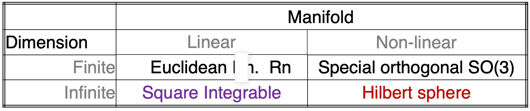
Methods in Functional Data Analysis are classified based on the type of manifold (linear or nonlinear) and the dimensionality or feature count of the space (finite or infinite). The categorization and examples of FDA techniques are demonstrated in the table below.
In Functional Data Analysis (FDA), the primary subjects of study are random functions, which are elements in a function space representing curves, trajectories, or surfaces. The statistical modeling and inference occur within this function space. Due to its infinite dimensionality, the function space requires a metric structure, typically a Hilbert structure, to define its geometry and facilitate analysis.
When the function space is properly established, a data scientist can perform various analytical tasks, including:
Computing statistics such as mean, covariance, and mode
Conducting classification and regression analyses
Performing hypothesis testing with methods like T-tests and ANOVA
Executing clustering
Carrying out inference
The following diagram illustrates a set of random functions around a smooth function X(tilde) over the interval [0, 1].
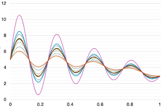
Fig. 1 Visualization of a random functions on Hilbert space
Methods in FDA are classified based on the type of manifold (linear or nonlinear) and the dimensionality or feature count of the space (finite or infinite). The categorization and examples of FDA techniques are demonstrated in the table below.
This article focuses on Hilbert space which is specific function space equipped with a Riemann metric (inner product).
Function Space
Let's consider a sample {x} generated by n Xi random functions as:
The function space L is a manifold of square integrable functions defined as
The Riemann metric tensor is defined for tangent vectors f and g is induced from and equal to the inner product <f, g>.
Manifolds
A full description of smooth manifolds is beyond the scope of this article. Manifolds and differential geometry is described in length in two previous articles Riemannian Manifolds:1 Foundations and Riemannian Manifolds: 2 Hands-on Hypersphere.
Here is a very brief review of the concepts:
A manifold is a topological space that, around any given point, closely resembles Euclidean space. Specifically, an n-dimensional manifold is a topological space where each point is part of a neighborhood that is homeomorphic to an open subset of n-dimensional Euclidean space. Examples of manifolds include one-dimensional circles, two-dimensional planes and spheres, and the four-dimensional space-time used in general relativity.
Smooth or Differential manifolds are types of manifolds with a local differential structure, allowing for definitions of vector fields or tensors that create a global differential tangent space.
A Riemannian manifold is a differential manifold that comes with a metric tensor, providing a way to measure distances and angles.
The tangent space at a point on a manifold is the set of tangent vectors at that point, like a line tangent to a circle or a plane tangent to a surface. Tangent vectors can act as directional derivatives, where you can apply specific formulas to characterize these derivatives.
In the context of smooth manifolds with a Riemannian metric, the exponential and logarithm maps provide a fundamental way to move between the manifold and its tangent spaces. These maps are crucial in optimization on manifolds, geometric deep learning, and Riemannian geometry, as they allow for computations to be performed in the tangent space, where linear algebra tools can be applied.
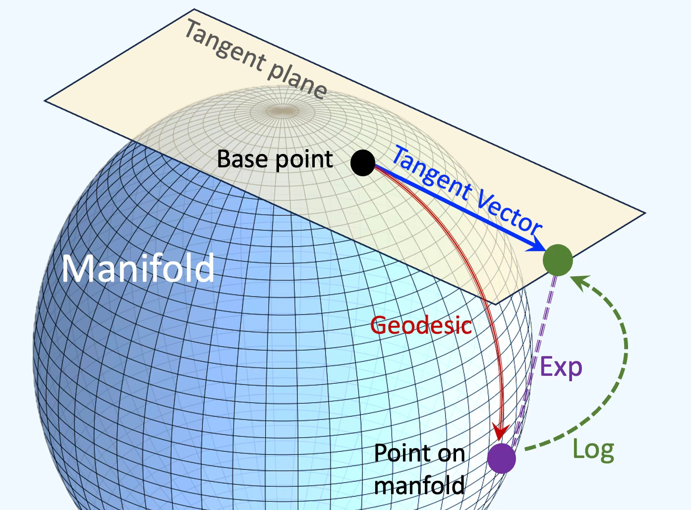
Fig. 2 Illustration of differential geometry elements on hypersphere; Manifold, Tangent vector, Geodesic, Exponential and Logarithm maps
Hilbert Sphere
Hilbert space is a type of vector space that comes with an inner product, which establishes a distance function, making it a complete metric space. In the context of functional data analysis, attention is primarily given to functions that are square-integrable [ref 5].
Hilbert space has numerous important applications:
Probability theory: The space of random variables centered by the expectation
Quantum mechanics:
Differential equations:
Biological structures: (Protein structures, folds,..)
Medical imaging (MRI, CT-SCAN,...)
Meteorology
The Hilbert sphere S, which is infinite-dimensional, has been extensively used for modeling density functions and shapes, surpassing its finite-dimensional equivalent. This spherical Hilbert geometry facilitates invariant properties and allows for the efficient computation of geometric measures.
The Hilbert sphere is a particular case of function space defined as:
The Riemannian exponential map at p from the tangent space to the Hilbert sphere preserves the distance to origin and defined as:
where ||f||E is the norm of f in the Euclidean space.
The logarithm (or inverse exponential) map is defined at point p, is defined as
⚙️ Hands-on with Python
Environment
Libraries: Python 3.11.8, Geomstats 2.7.0
Source code: Github.com/patnicolas/geometriclearning/geometry/manifold/function_space
To enhance the readability of the algorithm implementations, we have omitted non-essential code elements like error checking, comments, exceptions, validation of class and method arguments, scoping qualifiers, and import statements.
Geomstats is an open-source, object-oriented library following Scikit-Learn’s API conventions to gain hands-on experience with Geometric Learning. It is described in article Introduction to Geomstats for Geometric Learning
Implementation
🔎 Design
We will illustrate the various coordinates on the hypersphere space we introduced in the article Geometric Learning in Python: Manifolds
As a reminder, an hypersphere S of dimension d, embedded in an Euclidean space d+1 is defined as:
First we encapsulate the key components of a point on a manifold into a data class ManifoldPoint for convenience with the following attributes:
id A label a point
location A n dimension Numpy array
tgt_vector An optional tangent vector, defined as a list of float coordinate
geodesic A flag to specify if geodesic has to be computed.
intrinsic A flag to specify if the coordinates are intrinsic, if True, or extrinsic if False.

🔎 Functions Space Manifold
Let's develop a wrapper class named FunctionSpace to facilitate the creation of points on the Hilbert sphere and to carry out the calculation of the inner product, as well as the exponential and logarithm maps related to the tangent space.
Our implementation relies on Geomstats library [ref 6] introduced in Geometric Learning in Python: Manifolds
The function space will be constructed using num_domain_samples, which are evenly spaced real values within the interval [0, 1]. Points on a manifold can be generated using either the Geomstats HilbertSphere.random_point method or by specifying a base point, base_point, and a directional vector.

Let's generate a point on the Hilbert sphere using a random base point on the manifold and a 4 dimension vector.
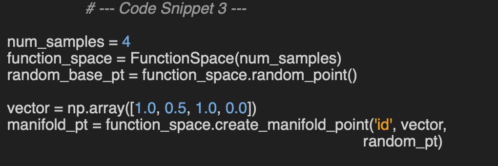
Manifold point:
Base point=[[0.13347 0.85738 1.48770 0.29235]],
Tangent Vector=[[ 0.91176 -0.0667 0.01656 -0.19326]],
No Geodesic,
Extrinsic
Evaluation
🔎 Inner Product
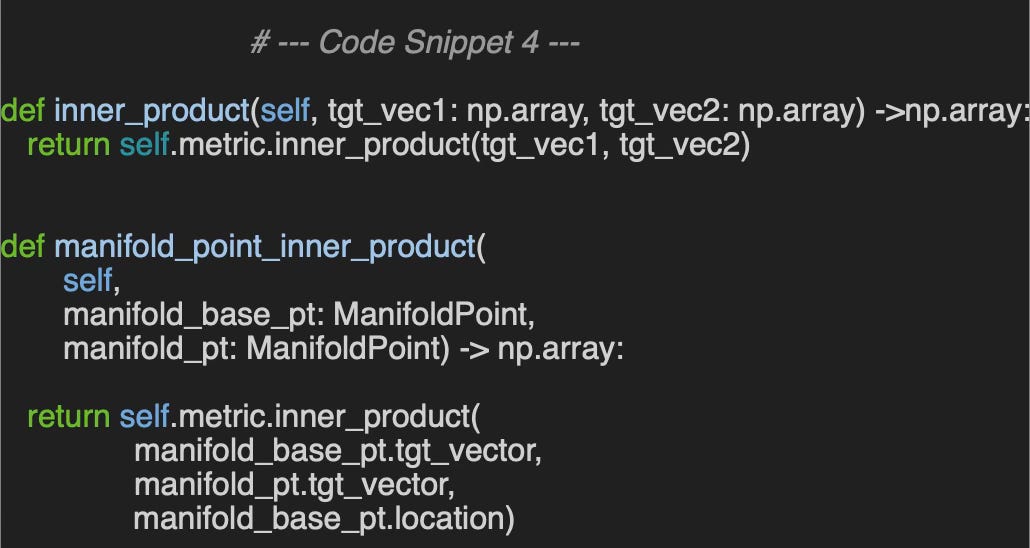
Let's wrap the formula (1) into a method. We introduce the inner_product method to the FunctionSpace class, which serves to encapsulate the call to self.metric.inner_product from the Geomstats method HilbertSphere.inner_product.
This method requires two parameters:
tgt_vec_1: The first vector in the tangent plane used in the computation of the inner product
tgt_vec_2: The second vector in the tangent plane used in the computation of the inner product
The second method, manifold_point_inner_product, adds the base point on the manifold without assumption of parallel transport. The base point is origin of both the tangent vector associated with the base point, manifold_base_pt and the tangent vector associated with the second point, manifold_pt.
Let's calculate the inner product of two specific numpy vectors in an 8-dimensional space, using our class, FunctionSpace and focusing on the Euclidean inner product and the norm on the tangent space for one of the vectors.
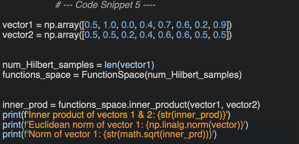
Output:
Inner product of vectors1 & 2: 0.2700
Euclidean norm of vector 1: 1.7635
Norm of vector 1: 0.6071
🔎 Exponential Map
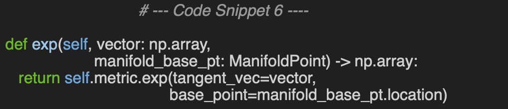
Let's wrap the formula (2) into a method. We introduce the exp method to the FunctionSpace class, which serves to encapsulate the call to self.metric.exp from the Geomstats method HilbertSphere.exp.
This method requires two parameters:
vector: The directional vector used in the computation the exponential map
manifold_base_pt: The base point on the manifold.
Let's compute the exponential map at a random base point on the manifold, for a numpy vector of 8-dimensional, using the class, FunctionSpace.
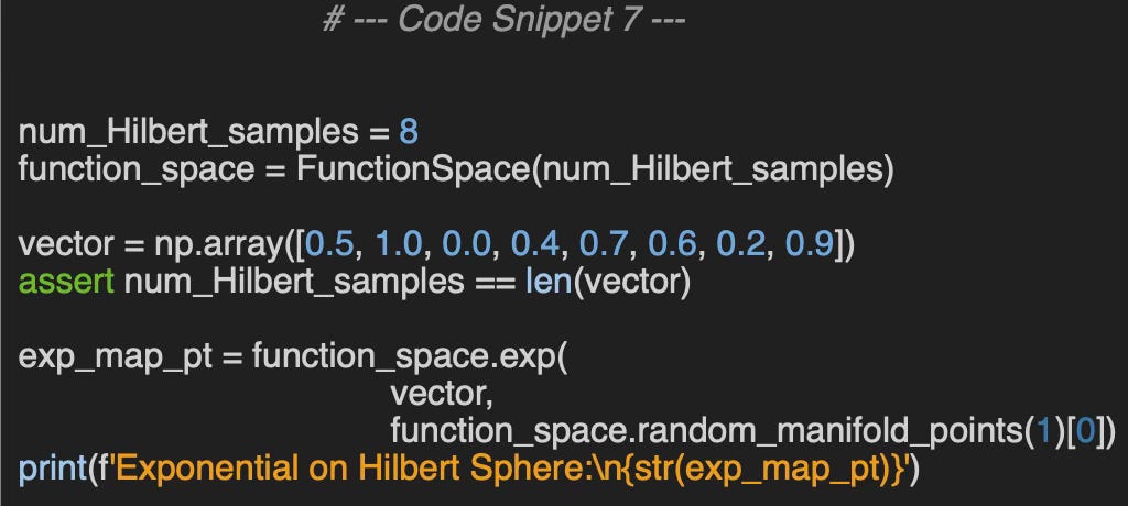
Output:
Exponential on Hilbert Sphere
[0.97514 1.6356 0.15326 0.59434 1.06426 0.74871 0.24672 0.95872]
🔎 Logarithm Map
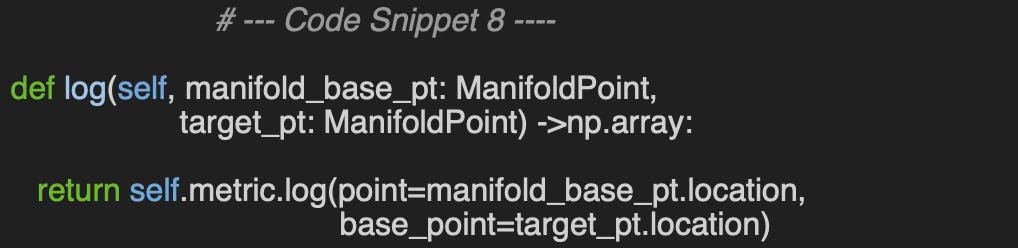
Let's wrap the formula (3) into a method. We introduce the log method to the FunctionSpace class, which serves to encapsulate the call to self.metric.log from the Geomstats method HilbertSphere.log.
This method requires two parameters:
manifold_base_pt: The base point on the manifold.
target_pt: Another point on the manifold, used to produce the log map.
Let's compute the exponential map at a random base point on the manifold, for a numpy vector of 8-dimensional, using the class, FunctionSpace.
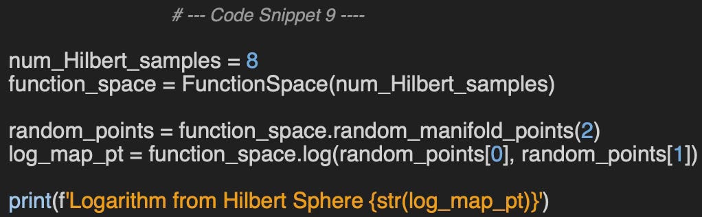
Output:
Logarithm from Hilbert Sphere
[1.39182 -0.08986 0.32836 -0.24003 0.30639 -0.28862 -0.431680 4.15148]
🧠 Key Takeaways
✅ Functional Data Analysis (FDA) is a robust approach for managing high-dimensional, continuous, and smooth data, enhancing modern machine learning algorithms with interpretability and feature-rich representations.
✅ We outline FDA methods in relation to linear and non-linear manifolds, distinguishing between finite and infinite dimensions.
✅ We utilize the Geomstats library to perform computations such as inner products, norms, and exponential and logarithmic maps on a Hilbert functional sphere.
📘 References
🛠️ Exercises
Q1: Observations can be classified based on their measurement process (e.g., repeated measurements, regular time intervals). Can you list the three main categories of observed data?
Q2: A function space is a manifold composed of which type of functions?
Continuous monotonic functions
Square-integrable functions
Differentiable functions
Exponential functions
Q3: What is the dimensionality of a Hilbert Sphere?
A 2-dimensional manifold
A manifold with infinite dimensions
A 3-dimensional manifold
Q4: Can you modify test code snippet #5 to compute the inner product using only the first half of each vector? What would be the value of `num_Hilbert_samples`, and what is the resulting inner product, inner_prod?
Q5: How is the inner product of two tangent vectors/functions <f, g> defined?
👉 Answers
💬 News & Reviews
This section focuses on news and reviews of papers pertaining to geometric deep learning and its related disciplines.
Paper review: Reliable Malware Analysis and Detection using Topology Data Analysis L. Nganyewou Tidjon, F. Khomh 2022
This paper introduces and evaluates three topological-based data analysis (TDA) techniques, to efficiently analyze and detect complex malware signature. TDA is known for its robustness under noise and with imbalanced datasets.
The paper first introduces the basic formulation of metric spaces, simplicial complexes, and homology before describing the 3 techniques for analysis.
TDA mapper
Persistence homology
Topological model analysis tool
These TDA techniques are compared to traditional features engineering (unsupervised) algorithms such as PCA or t-SNE using a False Positive Rate and a Detection Rate. The features are then used as input to various traditional ML classifiers (SVM, Logistic Regression, Random Forest, Gradient Boosting,).
The paper also covers CPU and memory usage analysis.
Conclusion: TDA mapper with PCA for feature extraction for extracting malware clusters as well as t-SNE to identify overlapping malware characteristics.As far as detection rate in supervised classification, Random Forest, XGBoost and GBM achieve a detection rate close to 100%. Basic understanding of machine learning and algebraic topology is required to benefit from the paper.
Patrick Nicolas is a software and data engineering veteran with 30 years of experience in architecture, machine learning, and a focus on geometric learning. He writes and consults on Geometric Deep Learning, drawing on prior roles in both hands-on development and technical leadership. He is the author of Scala for Machine Learning (Packt, ISBN 978-1-78712-238-3) and the newsletter Geometric Learning in Python on LinkedIn.