

Slimming the Graph Neural Network Footprint
Expertise Level ⭐⭐⭐

Practitioners of large-scale graph neural network training inevitably encounter GPU memory constraints. This article introduces and assesses critical training configurations for mitigating excessive GPU memory usage.


🎯 Why this matters
Purpose: Training transductive Graph Neural Networks—such as a Graph Convolutional Network (GCN) for node classification—can be highly GPU-memory intensive. Beyond general Python/PyTorch best practices, combining multiple training-time techniques helps prevent out-of-memory failure
Audience: Data scientists and engineers building models for node/graph classification or link prediction on very large graph data set.
Value: Evaluate training configurations for Graph Convolutional Networks that minimize GPU memory usage (on MPS or CUDA) by leveraging Python decorators.
🎨 Modeling & Design Principles
⚠️ The recommendations—and their evaluations—primarily target Graph Neural Networks built with PyTorch and PyTorch Geometric libraries. Applicability to other frameworks may vary.
Overview
Training GNNs (notably in transductive regimes) often demands significant memory. Effective mitigation blends methods from:
Python language practices
Machine learning models and training
PyTorch & PyTorch Geometric tooling
This article focuses on some important memory allocation management techniques related to model training in PyTorch and PyTorch Geometric. But first, let’s briefly review common memory optimization approach specific to Python and PyTorch library.
Python
I highly recommend “Effective Python: 59 Specific Ways to Write Better Python” by Brett Slatkin and the PEP 8 writing style standard.
A partial list includes
Using generator expression instead of loop or comprehensive lists
Leveraging immutability of tuples
Use slots whenever possible (e.g., @dataclass(slots=True)
Restricted memoization by capping cache size (lru_cache)
Segment I/O operation in accessing large binary files (e.g. mmap)
Delete object within method before going out of scope.
📌 It is highly recommended to use a memory profiler to make a line-by-line or statement-by-statement analysis of memory consumption for Python functions - Examples are listed in Appendix.
PyTorch
Here is a partial checklist to cut training memory usage in PyTorch on CUDA/GPU
autocast (torch.bfloat16) and Graph Scaler (torch.cuda.amp.GradScaler)
Activation checkpointing
Micro-batching and grad accumulation
In-place activation (e.g., nn.ReLU(inplace = True)
Deactivate cache (cache.detach())
pin_memory=True and non_blocking for device (e.g., cuda(non_blocking=True)
⚠️ Some of the recommendations are specific to CUDA device. Other devices, supported by PyTorch such as Metal Performance Shaders (MPS) backend may require different remedial techniques using alternative torch modules.
Mitigation Techniques
Now let’s investigate how to mitigate excessive memory consumption during training and validation of graph neural networks.
Reduce number and size of hidden layers: As cost of activations increases quadratically in some message-passing stacks (e.g., size of hidden layer reduced from 256 nodes to 128)
Mixed-Precision: 16 or 32-bit float data type for network weights whenever possible (e.g., PyTorch autocast). You may store node features in float16 on disk [ref 1].
⚠️ It is recommended to keep 32-bit float for the computation of the loss.
Use pin_memory=True. While the GPU trains on the first mini-batch, the CPU preloads the second to the device, so the GPU has data ready the moment it finishes and never sits idle [ref 2].

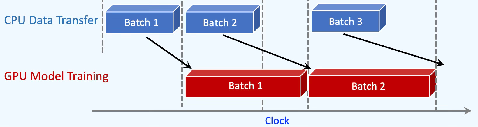
Fig. 1 Illustration of asynchronous data transfer from CPU to GPU
Reduce the number of workers in data loaders: A large number of workers can increase memory. Use num_workers=4 as a starting point.
Activation checkpointing: It allows to cut activation memory by up to 50% at the cost of extra compute. The memory reduction is square root of the memory required to process all neural layers. Storing all the intermediate activations in memory is not required. Instead, you may store a few of them and recomputing the rest when needed.
A common solution to break the large neural network into chunks or segments and process only the first layer in each segment as illustrated below [ref 3]:
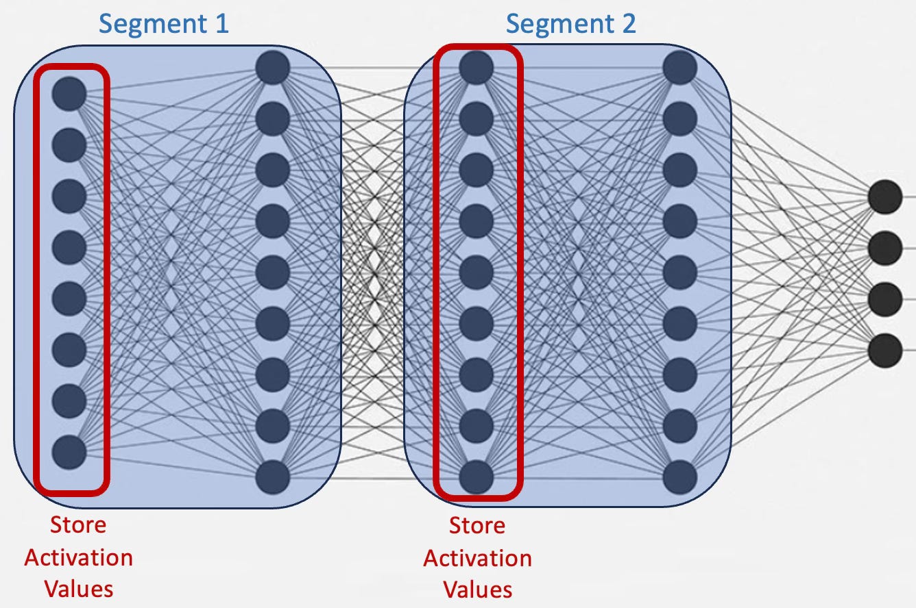
Fig. 2 Illustration of segmentation of a neural networks for activation checkpointing
Feature pruning: Unsupervised feature reduction technique such as Principal Component Analysis, Singular Value Decomposition or Manifold Learning reduces the dimension of the input data.
Features importance: Drop feature that has limited impact on the quality of prediction.
Memory management on GPU: Unload variables from GPU to CPU when not needed (e.g., data = data.cpu())
Cache management: Clear the cache after each key operation (e.g. torch.cuda.empty_cache() or torch.mps.empty_cache() )
Neighbor loader and sampler: The most recommended PyTorch Geometric data loaders are [ref 4]
NeighborLoader with small fanouts for node classification
LinkNeighborLoader with modest negative sampling for link prediction
GraphSAINT family of graph data loaders for stochastic sampling
Batch size: Memory usage during training increases with the size of batch of sampled nodes in aggregating messages.
Training configuration: Remedial techniques associated with generic deep learning models such as gradient accumulation, zero gradient for each batch (optimizer.zero_grad(set_to_none=True)), restrict retain_graph=True to training or
torch.no_grad() for validation apply.
⚙️ Hands‑on with Python
Environment
Libraries: Python 3.11.8, PyTorch 2.1.0, PyTorch Geometric 2.5.0
Source code memory usage decorator:
geometriclearning/util/monitor_memory_device.py
Evaluation code: geometriclearning/play/gnn_memory_monitor_play.py
The source tree is organized as follows: features in python/, unit tests in tests/,and newsletter evaluation code in play/.
To enhance the readability of the algorithm implementations, we have omitted non-essential code elements like error checking, comments, exceptions, validation of class and method arguments, scoping qualifiers, and import statements.
⚠️ Some sampling methods in PyTorch Geometric rely on additional modules: torch-sparse, torch-scatter, torch-spline-conv, and torch-cluster. These are dependencies oftorch-geometric but they may not be compatible with the latest versions of PyTorch, particularly across different operating systems.
For macOS, we recommend the following version setup for best compatibility:
Python: 3.11.8
PyTorch: 2.1.0
torch-geometric: 2.6.1
torch-sparse: 0.6.18
torch-scatter: 2.1.2
torch-spline-conv: 1.2.2
torch-cluster: 1.6.3
These modules currently support only CPU and CUDA execution — MPS (Metal) is not supported.
🔎 Decorators
We’ll leverage a powerful Python feature—decorators—to automate collecting and reporting memory usage [ref 5].
We implemented decorator for the CUDA, MPS and CPU (not shown) target devices.
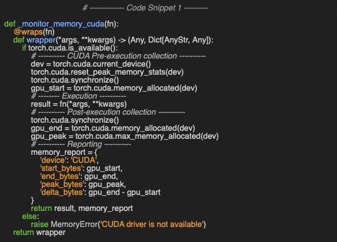
The decorator for Nvidia GPU/CUDA relies on the torch.cuda module [ref 6]. In its simplest form, the annotator, _monitor_memory_cuda collects memory at beginning, end of execution as well as peak usage.
The annotator for Mac MPS, _monitor_memory_mps follows the same logic as the annotator for Nvidia GPU and leverages the torch.mps module [ref 7]. It supports the collection of memory usage at the device (MPS) level.
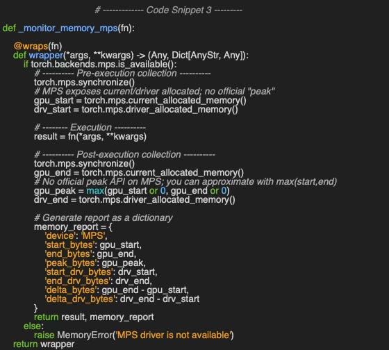
We tie the various annotators to create a dynamic annotator monitor_memory_device as illustrated in code snippet 3.
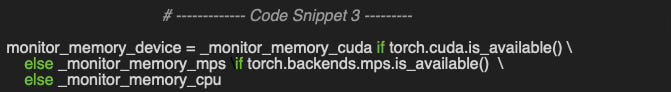
The full implementation of the decorator is available on Github at geometriclearning/util/monitor_memory_device.py
We introduced the training of a Graph Convolutional Network in a previous article [ref 8] with the source code on Github geometriclearning/play/gnn_training_play.py
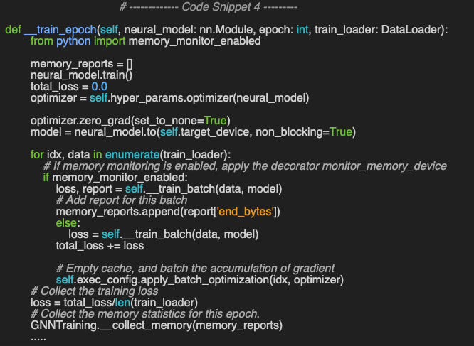
The training loop described in a previous article [ref 8] has to be modified to enable the collection of memory parameters as illustrated in code snippet 4.
📌 Contrary to GCN and GAT, GraphSAGE does not rely of torch.scatter and therefore is compatible with the latest very versions of PyTorch.
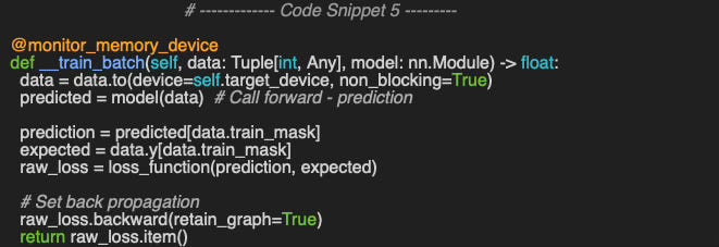
Finally, the execution of the back propagation for each batch is described in code snippet 5.
👉 The evaluation code available at geometriclearning/play/gnn_memory_monitor_play.py
📈 Evaluation
Setup
Processor: V100 (alt. M4 Max)
Software: Cuda 11.7 (alt. MPS)
Dataset: Flickr
PyG data loader/node neighbors sampler: NeighborLoader
Graph Neural Network Architecture: Graph Convolutional Network (Transductive)
Application: Node classification
📌 We use a Graph Convolutional Network (GCN) in our evaluation for two reasons:
it maintains continuity with prior work, and
as a transductive method, it loads the entire graph into memory.
We leverage the same model and training parameters used in previous articles Graph Convolutional or SAGE Networks? , Revisiting Inductive Graph Neural Networks and Plug & Play Training of Graph Convolutional Networks. We include the JSON configuration for the training and Graph Convolutional Network used in the evaluation in the Appendix (Appendix: Training Configuration)
Results
Size of hidden Layers
Let’s quantify the impact of the size of hidden layers on the memory consumption. Our evaluation model is a Graph Convolutional Network with a single hidden layer.
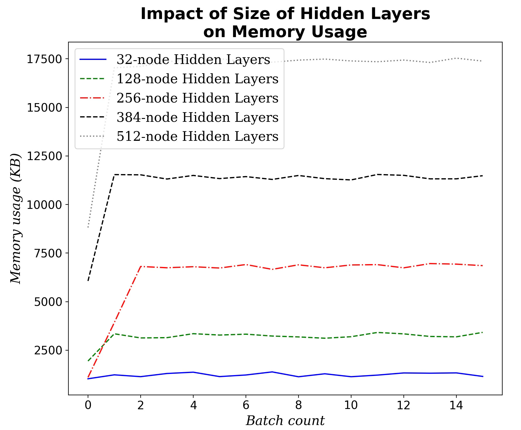
Fig. 3 Impact of the size of the single hidden layer on memory consumption during training
As expected, the memory usage increases proportionally with the number of nodes in the hidden layers.
📌 We did not use any pruning or regularization during the various tests.
GPU Transfer Memory
Let’ evaluate the best configuration to reduce GPU idle periods by preloading batches via asynchronous CPU-to-GPU transfers (pin_memory=True vs. pin_memory=False)
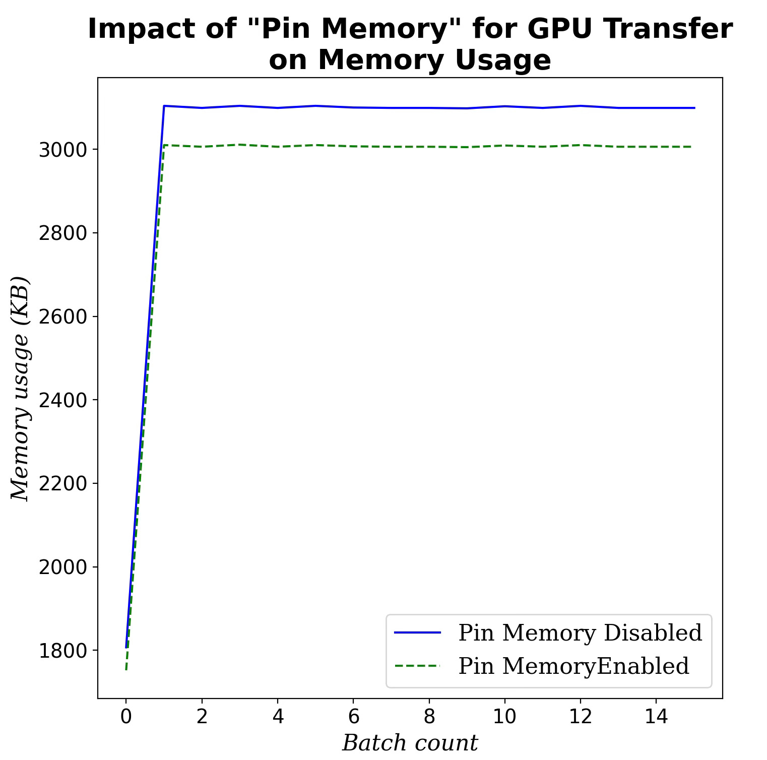
Fig. 4 Impact of the optimization of data transfer to GPU (pin_memory) on memory consumption during training
Clearly setting pin_memory=True to optimize the transfer of input data from CPU to GPU has a positive although limited impact.
Mixed Precision Autocast
Our default data type for the weight of the Graph Convolutional Network is 64-bit float. We evaluate the performance improvement with 32-bit and 16-bit floating point for the model parameters in forward pass and backward computation.
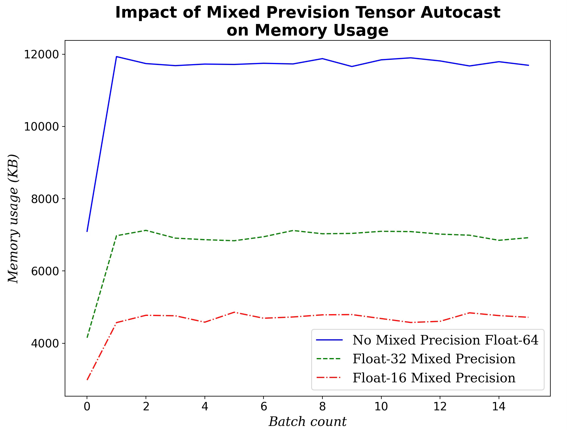
Fig. 5 Impact of the 16 & 32 bit float mixed-precision on memory consumption during training
The memory usage dropped significantly when switching from 64-bit to 32 and 16-bit. Moreover memory usage decreases is almost proportional along with the number of bits used for model weights:
64 bit → 32 bit: 43.4% reduction
64 bit → 16 bit: 63.6% reduction
Number of Workers in Node Sampling
As noted earlier, reducing the number of workers used for node sampling in message aggregation will likely lower memory usage during training.
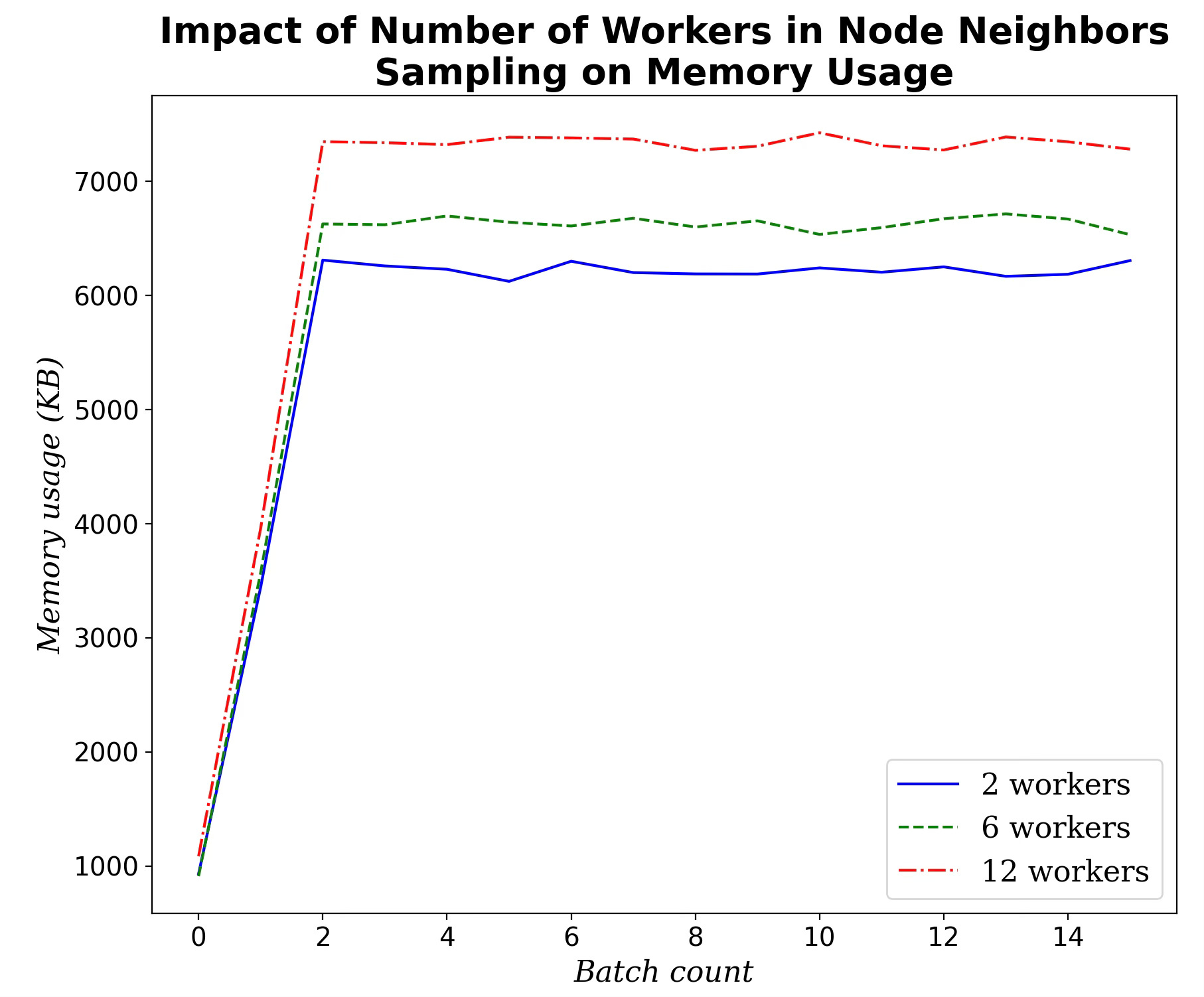
Fig. 6 Impact of the number of worker in PyG graph data loader on memory consumption during training
Clearly, the improvement in memory usage is somewhat marginal.
Neighborhood Sampling
Finally, we examine how PyTorch Geometric’s NeighborLoader sampling settings affect memory usage.
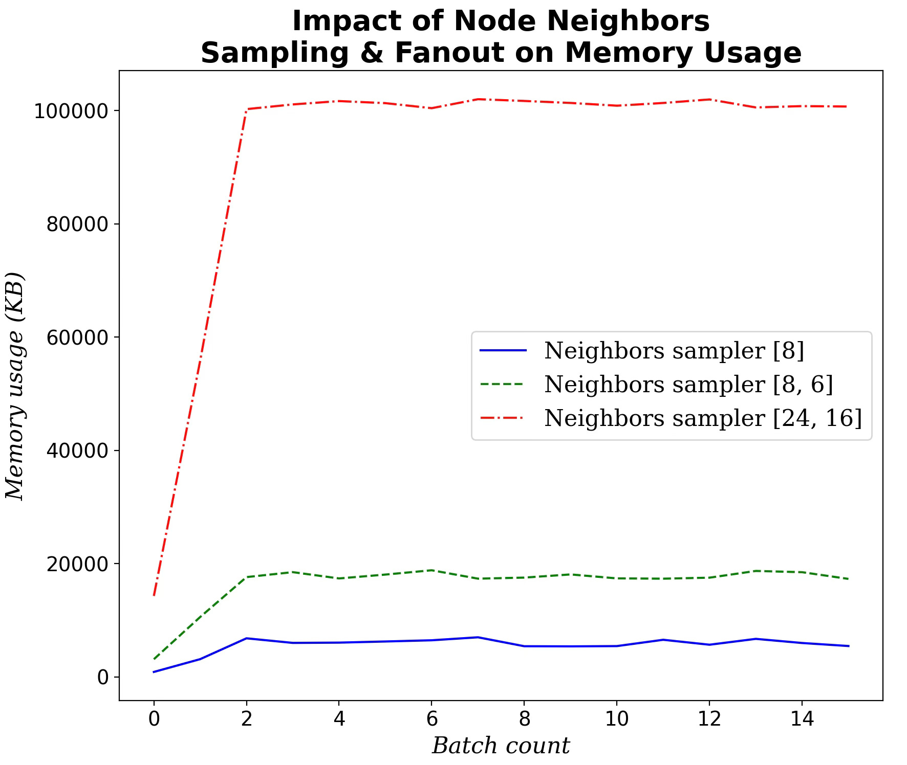
Fig. 7 Impact of the configuration of node neighbors sampling (hops, fanout) on memory consumption during training
Increasing the number of sampled neighbors for each hop and fanout has a very significant impact of memory usage.
⚠️ This evaluation focuses on training-time memory usage and does not assess its effect on node-classification quality. In practice, memory optimizations often reduce a model’s performance.
🧠 Key Takeaways
✅ Neighbor sampling dominates memory: In GCN training, the graph data loader’s neighbor-sampling strategy has the largest impact on memory usage.
✅ Data-transfer tweaks help little: Using pin_memory=True or reducing the number of data-loader workers yields only marginal memory savings.
✅ Mixed precision helps: As in standard deep learning, mixed-precision training meaningfully lowers memory consumption.
✅ Fewer nodes ≠ pruning, still big savings: Even without pruning, reducing the number of nodes (our model has a single hidden layer) substantially cuts memory use.
📘 References
Automatic Mixed Precision examples PyTorch Documentation
When to set pin_memory to true? K. Zhong - PyTorch Documentation
How Activation Checkpointing enables scaling up training deep learning models - Medium Y. Beer, O. Bar - Medium
Demystifying Graph Sampling & Walk Methods Hands-on Geometric Deep Learning, 2025
Decorators in Python Geeks for Geeks, 2025
Reference API: torch.cuda PyTorch documentation
MPS backend PyTorch documentation
Plug & Play Training of Graph Convolutional Networks Hands-on Geometric Deep Learning, 2025
🧩 Appendix
Memory Profiler
Below you can see how to use memory_profiler within your Python script:
Decorate the function you want to profile with @profile
Run the script by passing the option -m memory_profiler to load the memory_profiler module.
Training Configuration
Here is the configuration of the training of the Graph Convolutional Network for node classification on PyTorch Geometric Flickr dataset. As described in the previous article, Plug & Play Training of Graph Convolutional Networks the configuration is loaded as a JSON descriptor.
training_attributes = {
   ‘dataset_name’: ‘Cora’,
        # Model training Hyperparameters
   ‘learning_rate’: 0.0012,
   ‘batch_size’: 32,
   ‘loss_function’: nn.CrossEntropyLoss(label_smoothing=0.08),
   ‘momentum’: 0.95,
   ‘weight_decay’: 1e-3,
   ‘weight_initialization’: ‘Kaiming’,
   ‘is_class_imbalance’: True,
   ‘class_weights’: class_weights,
   ‘hidden_channels’:128,
   ‘tensor_mix_precision’: float16,
   ‘checkpoint_enabled’: True,
   ‘epochs’: epochs,
         # Performance metrics
   ‘metrics_list’: [’Accuracy’, ‘Precision’, ‘Recall’, ‘F1’,
                    ‘AucROC’, ‘AucPR’],
   ‘plot_parameters’: { .... }
 }
Model Configuration
Here is the configuration of the Graph Convolutional Network for node classification on PyTorch Geometric Flickr dataset. As described in the previous article, Plug & Play Training of Graph Convolutional Networks the configuration is loaded as a JSON descriptor.
{
   ‘model_id’: ‘MyModel’,
   ‘gconv_blocks’: [
      {
        ‘block_id’: ‘conv_block_1’,
        ‘conv_layer’: GraphConv(in_channels=num_node_features,
                                out_channels=hidden_channels),
        ‘num_channels’: hidden_channels,
        ‘activation’: nn.ReLU(),
        ‘batch_norm’: None,
        ‘pooling’: None,
        ‘dropout’: 0.25
      },
         {
        ‘block_id’: ‘conv_block_2’,
        ‘conv_layer’: GraphConv(in_channels=hidden_channels,
                                out_channels=hidden_channels),
        ‘num_channels’: hidden_channels,
        ‘activation’: nn.ReLU(),
        ‘batch_norm’: None,
        ‘pooling’: None,
        ‘dropout’: 0.25
      },
   ],
   ‘mlp_blocks’: [
      {
        ‘block_id’: ‘mlp_block’,
        ‘in_features’: hidden_channels,
        ‘out_features’: num_classes,
        ‘activation’: None,
        ‘dropout’: 0.0
      }
   ]
 }
Training Output
Here is a typical output of a training as described in article Plug & Play Training of Graph Convolutional Networks
💬 News & Reviews
This section focuses on news and reviews of papers pertaining to geometric deep learning and its related disciplines.
Paper Review: HLSAD: Hodge Laplacian-based Simplicial Anomaly Detection F. Frantzen, M. T. Schaub - RWTH Aachen University, Department of Computer Science - 2025
This paper examines the limitations of temporal/dynamic GNNs for anomaly detection and proposes using the Hodge Laplacian of a simplicial complex—a richer representation of node interactions, defined as the sum of the up- and down-Laplacians. Graphs are lifted to simplicial complexes via clique or neighborhood expansions. After introducing incidence matrices and weighted Hodge Laplacians, the authors distinguish between event and change anomalies.
Method
1. Compute Hodge Laplacians over a time series of simplicial complexes.
2. From each Laplacian, extract the top nn singular values (dimensionality reduction).
3. Detect anomalies by comparing the current feature vector against short- and long-term trends using a sliding window.
4. Score anomalies as the maximum deviation across the two horizons.
Evaluation
Evaluations on stochastic block–model graphs and the MIT Reality Mining / UCI Online Message datasets show that the method flags all relevant anomalies using as few as 40 singular values.
Reader classification rating
⭐ Beginner: Getting started - no knowledge of the topic
⭐⭐ Novice: Foundational concepts - basic familiarity with the topic
⭐⭐⭐ Intermediate: Hands-on understanding - Prior exposure, ready to dive into core methods
⭐⭐⭐⭐ Advanced: Applied expertise - Research oriented, theoretical and deep application
⭐⭐⭐⭐⭐ Expert: Research , thought-leader level - formal proofs and cutting-edge methods.
Patrick Nicolas is a software and data engineering veteran with 30 years of experience in architecture, machine learning, and a focus on geometric learning. He writes and consults on Geometric Deep Learning, drawing on prior roles in both hands-on development and technical leadership. He is the author of Scala for Machine Learning (Packt, ISBN 978-1-78712-238-3) and the newsletter Geometric Learning in Python on LinkedIn.