Revisiting Inductive Graph Neural Networks

Expertise Level ⭐⭐⭐

Sep 03, 2025

GraphSAGE addresses limitations we encountered with Graph Neural Networks in prior articles—namely, it offers dynamic, learnable aggregation and an inductive training strategy.

🎯 Why this Matters
🎨 Modeling & Design Principles
Overview
Message Passing & Aggregation
Transductive vs. Inductive Graph Networks
⚙️ Hands-on with Python
Environment
🔎 Graph SAGE block
🔎 Graph SAGE Model
🔎 Training & Validation
Configuration
📈 Evaluation
Datasets
Performance Metrics
Graph Sub-sampling & Latency
🧠 Key Takeaways
🛠️ Exercises
📘 References
💬 News & Reviews

🎯 Why this matters

Purpose: Previous articles relied on Graph Convolutional Networks (GCNs). Though computationally efficient, they require full-graph training and use non-learnable aggregators. Graph SAGE models address some of these limitations.

Audience: Data scientists and machine learning engineers learning or building, training, validating and tuning graph neural networks

Value: Learn about GraphSAGE networks and the hyperparameters that shape performance—subgraph sampling size, layer depth, and neighborhood sampling.

🎨 Modeling & Design Principles

Overview

In previous issues, we introduced Graph Neural Networks [ref 1] and evaluated Graph Convolutional Networks (GCNs) [ref 2]. We now turn our attention to GraphSAGE (Graph Sample and Aggregate) — a framework designed for inductive node representation learning on very large graphs [ref 3].

The term inductive refers to the model’s ability to learn a generalizable function that applies to nodes, edges, or even entire graphs that were not seen during training.

One of the key advantages of this inductive approach is that it eliminates the need to train on the entire graph, enabling scalability.

The core steps of GraphSAGE are:

Sample a fixed number of neighbors for each node
Aggregate the features of the sampled neighbors (e.g., by mean or pooling)
Concatenate the aggregated features with the node’s own features
Update the node embeddings through stacked layers

The typical applications are:

Large-scale social networks (Flickr, Reddit)
Recommendation systems
Dynamic node classification

Message Passing & Aggregation

As described in [ref 1], message passing and aggregation underpin GNNs; we summarize and illustrate them here

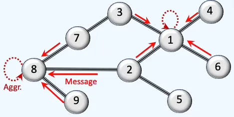
Fig. 1 Illustration Message-passing and Aggregation in Graph Neural Networks

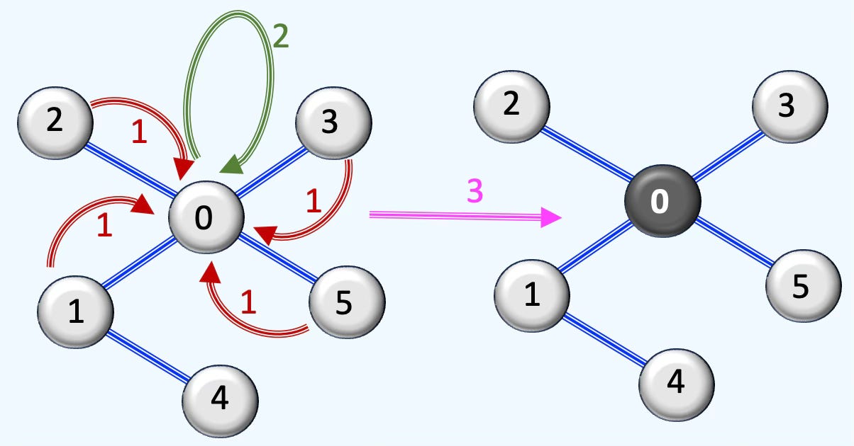
Fig. 2 Illustration of the 3 steps in processing a graph through a graph SAGE neural layer

As shown in Figure 2, a neural layer processes the graph in three stages:

Message collection: Node 0 gathers information from its neighboring nodes.
Aggregation: The collected messages are combined using operations such as sum, mean, or pooling.
Feature update: The node’s own features are updated based on the aggregated information.

The generic message passing model is the most expressive design making it suitable for complex modeling such as dynamic systems, proteins generation at a high computational cost and memory consumption [ref 4].

\(\begin{matrix} \psi\left( h_{j}^{(k)} \right) = W. h_{j}^{(k)}+ b \ \ \ Trainable \ function \\ \mu_{ij}=\psi \left( h_{i}^{(k)}, h_{j}^{(k)} \right) \ \ \ \ Feature \ vector \ nodes \ i \ j\\ h_{i}^{(k+1)} =\Phi \left( \bigwedge_{ij} \left( h_{j}^{(k)}, \bigoplus_{j\in N_{i}}\psi\left( h_{i}^{(k)}, h_{j}^{(k)} \right) \right) \right) \\ \bigwedge: Concatenator \ \ \ \ \ \ \ \ \ \ \ \ \ \ \ \ \ \ \ \ \ \ \ \ \ \ \ \ \ \ \ \ \ \ \ \ \ \ \ \ \ \ \ \ \ \ \ \ \\ \bigoplus: Aggregator \ \ \ \ \ \ \ \ \ \ \ \ \ \ \ \ \ \ \ \ \ \ \ \ \ \ \ \ \ \ \ \ \ \ \ \ \ \ \ \ \ \ \ \ \ \ \ \ \ \ \ \ \ \end{matrix}\)

µ_ij is a feature vector that describes the interaction of node i with node j.·
N_iis the 1-hop neighborhood of i (excluding i)
w_ijare unlearned weights, usually depending only on the local graph topology and which encode the connection strength between pairs of nodes.

Transductive vs. Inductive Graph Networks

Graph Convolutional Networks (GCNs) were reviewed in [ref 2]. A straightforward way to characterize GraphSAGE is by contrasting it with GCNs: Graph Convolutional Networks are transductive models while GraphSAGE is an instance of a inductive model.

In a nutshell:

Transductive GNNs learn using the entire target graph (including test nodes/edges) during training and predict labels for those specific nodes/edges.
Inductive GNNs learn a function (message-passing/aggregation rules) that transfers to unseen nodes or entirely new graphs at test time.

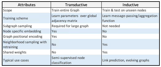
Table 1. Comparison of Transductive Graph Networks (e.g., GCN) and Inductive Graph Networks (e.g., GraphSAGE)

Table 1 underscores the dynamic, inductive character of GraphSAGE as its primary benefit.

⚙️ Hands‑on with Python

Environment

Libraries: Python 3.12.5, PyTorch 2.5.0, Numpy 2.2.0, Networkx 3.4.2, TopoNetX 0.2.0
Source code:
Features: geometriclearning/deeplearning/model/graph/graph_sage_model.py
Evaluation: geometriclearning/play/graph_sage_model_play.py
The source tree is organized as follows: features in python/, unit tests in tests/, and newsletter evaluation code in play/.
To enhance the readability of the algorithm implementations, we have omitted non-essential code elements like error checking, comments, exceptions, validation of class and method arguments, scoping qualifiers, and import statements.

Many deep learning models consist of numerous components, often with repeated structures. Developing and evaluating models in PyTorch can be streamlined by utilizing a library of predefined, tested, and reusable components: Neural Blocks.

🔎 Graph SAGE Block

⏭️ This section guides you through the design and code—skip if you only want results.

Neural blocks have been introduced and described in detail in a previous article [ref 5].

First, we define a GraphSAGEBlock class for the GraphSAGE network, which bundles together (as defined in the default constructor in code snippet 1)

SAGE convolutional layer: graph_SAGE_layer
Batch normalization module: batch_norm_module
Activation function: activation_module
Dropout module for training-time regularization: dropout_module

The class GraphSAGEBlock provides an alternative and more convenient constructor, build using a declarative format (dictionary/JSON) as input (as described in Configuration section).

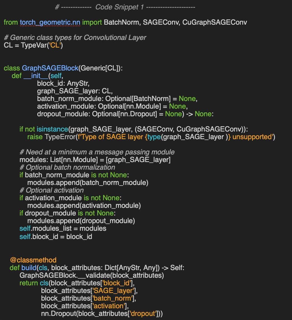
In this configuration, the constructor allows only two type of SAGE convolutional layer: SAGEConv & CuGraphSAGEConv

The alternative constructor, build instantiates a GraphSAGE block from a JSON-formatted configuration string.

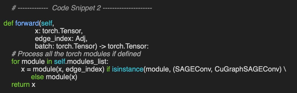
📌 The order in which PyTorch modules are added in the constructor determines their execution order in forward (see code snippet 2)

The forward method for the SAGE block iterates simply through all its modules (code snippet 2). The method invokes the forward method with the edge indices for module representing a neural layer of type SAGEConv or CuGraphSAGEConv.

🔎 Graph SAGE Model

⏭️ This section guides you through the design and code

Creating deep learning models is simple and intuitive. It consists of assembling predefined neural blocks [ref 6].

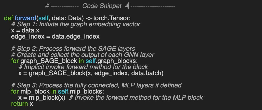
In the case of Graph SAGE network, a GraphSAGEModel is assembled using an ordered sequence of SAGE blocks, graph_SAGE_blocks and optionally, one or more fully connected, multi-perceptron blocks, mlp_blocks.

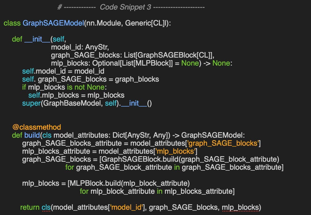
As with the Graph Neural Block, the build constructor instantiates a GraphSAGE model from a JSON-formatted configuration string.

The implementation of the forward method is pretty straightforward: it iteratively invokes the forward method for each SAGE convolution block (step 2) and then the multi-layer perception blocks if any are defined (step 3) in code snippet 4.

🔎 Training & Validation

⏭️ This section guides you through the design and code

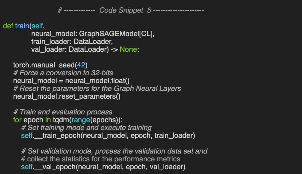
The training/validation method, train of class GraphSAGEModel, takes 3 arguments as illustrated in code snippet 5.

neural_model: The model as a torch.nn.Module
train_loader: Data loader for the training data set
val_loader: Data loader for the validation data set

In PyTorch Geometric, data loaders are closely linked to the sampling strategy used to determine the nodes from which each node gathers and aggregates information [ref 7].
These specialized data loaders for graph neural networks were discussed in detail in a previous article [ref 8].

The execution of training for each epoch relies on the batching of graph nodes feature data, similar to any other neural network (code snippet 6).

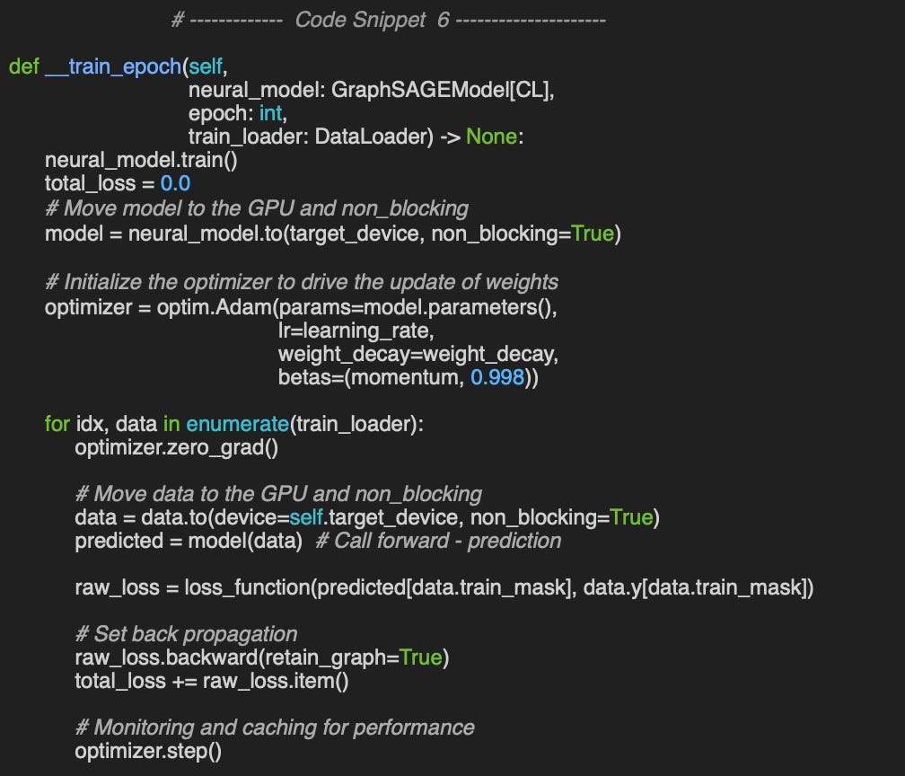
We select the Adam optimizer to compute the gradient of the loss function per weights. The predicted data, predicted, and labeled data, data.y are extracted through the train_mask defined for any given PyTorch Geometric data set used in this article.

📌 I did not describe the implementation of the validation method __val_epoch as it is very similar to the training method for each epoch and can be viewed on Github.

The Cora dataset is loaded via PyTorch Geometric’s Planetoid class [ref 8]. The test runs in five stages (code snippet 7):

load the graph,
instantiate the model,
create a GNNTraining instance,
build train/validation data loaders with optional graph subsampling,
train and validate.

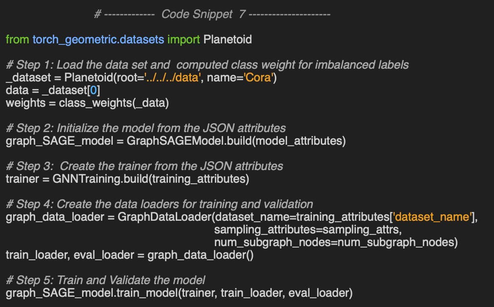
Graph data loaders are covered in detail in a previous article [ref 8]. The num_subgraph_nodes parameter sets how many nodes are randomly sampled from the original graph when it’s large.

The configuration for the model, model_attributes, training/validation, training_attributes and node sampling method, sampling_attributes are implemented as dictionaries and declared in JSON string formats.

The class GNNTraining has been introduced in previous article, [ref 2].

Configuration

The training_attributes JSON string specifies all relevant hyperparameters, performance metrics, and plot configurations required for training and evaluating the model.

training_attributes = {
   'dataset_name': 'Cora',
        # Model training Hyperparameters
   'learning_rate': 0.0012,
   'batch_size': 32,
   'loss_function': nn.CrossEntropyLoss(label_smoothing=0.08),
   'momentum': 0.95,
   'weight_decay': 1e-3,
   'weight_initialization': 'Kaiming',
   'is_class_imbalance': True,
   'class_weights': class_weights,
   'epochs': epochs,
         # Performance metrics
   'metrics_list': ['Accuracy', 'Precision', 'Recall', 'F1', 
                    'AucROC', 'AucPR'],
   'plot_parameters': {
           ....
    }
 }

As the name implies, the model_attributes JSON representation outlines the different blocks, layers, and activation modules that compose the model.

model_attributes = {
  'model_id': title,
       # Graph SAGE blocks
  'graph_SAGE_blocks': [
    {
      'block_id': 'SAGE Layer 1',
      'SAGE_layer': SAGEConv(in_channels =_dataset[0].num_node_features, 
                             out_channels=hidden_channels),
      'num_channels': hidden_channels,
      'activation': nn.ReLU(),
      'batch_norm': None,
      'dropout': 0.25
    },
    {
      'block_id': 'SAGE Layer 2',
      'SAGE_layer': SAGEConv(in_channels=hidden_channels, 
                             out_channels=hidden_channels),
      'num_channels': hidden_channels,
      'activation': nn.ReLU(),
      'batch_norm': None,
      'dropout': 0.25
    }
  ],
        # Fully connected blocks
  'mlp_blocks': [
    {
      'block_id': 'Node classification block',
      'in_features': hidden_channels,
      'out_features': _dataset.num_classes,
      'activation': None
    }
 ]
}

Finally, the sampling_attributes JSON string defines the strategy for selecting a node’s neighbors from which it will receive and aggregate messages. We selected by default the Node Neighborhood Sampler described in [ref 8]

sampling_attributes = {
  'id': 'NeighborLoader',
  'num_neighbors': [12, 8],
  'batch_size': 32,
  'replace': True,
  'num_workers': 4
}

📈 Evaluation

Our goal is to understand:

The performance impact of model choices, focusing on i) neighbor sampling in message passing/aggregation (using an arbitrary configuration for illustration) and ii) number of convolutional layers in the SAGE model.
How the size of the sampled subgraph affects latency and node-classification performance

Datasets

We select the small size Cora and PubMed graph data set for the first tests, and the larger Flickr graph for the second test.

Cora: A standard benchmark dataset for semi-supervised node classification, containing 2,708 nodes (scientific publications) and 5,429 edges (citations). Each node is described by a 1,433-dimensional feature vector. This dataset is also included in torch_geometric.datasets.Planetoid class collection.

PubMed: Consists of 19,717 scientific publications from the PubMed database, each pertaining to diabetes and classified into one of three classes. The citation network includes 44,338 edges, and each node has a 500-dimensional feature vector. This dataset is also included in torch_geometric.datasets.Planetoid class collection.

Flickr: Contains descriptions and common properties of 89,250 images along with 899.756 edges and a 500-dimensional feature vector. It is defined in torch_geometric.datasets.Flickr class.

Performance metrics

Neighborhood Mode Sampling Parameters

The first experiment measures Precision, Recall, Accuracy, F1, AUC-ROC, and AUC-PR versus the number of hops and the number of neighbors sampled for aggregation:

[6, 3] # 6 neighbors first hop → 3 neighbors each second hop
[12, 8] # 12 neighbors first hop → 8 neighbors each second hop
[12, 12, 6] # 12 neighbors first hop → 12 neighbors each second hop → 6 neighbors each third hop

Cora dataset configuration:

Sampling: {'id': 'NeighborLoader', 'num_neighbors': [6, 3], 
           'batch_size': 32, 'replace': True, 'num_workers': 4}
Number graphs: 1
Number nodes: 2708
Number features: 1433
Number classes: 7
Is directed: False
Has loop: False
Training nodes: 140
Validation nodes: 500
Subgraph coverage: 1.000

Here is an example of performance metrics for 6 x 3 neighboring node sampling

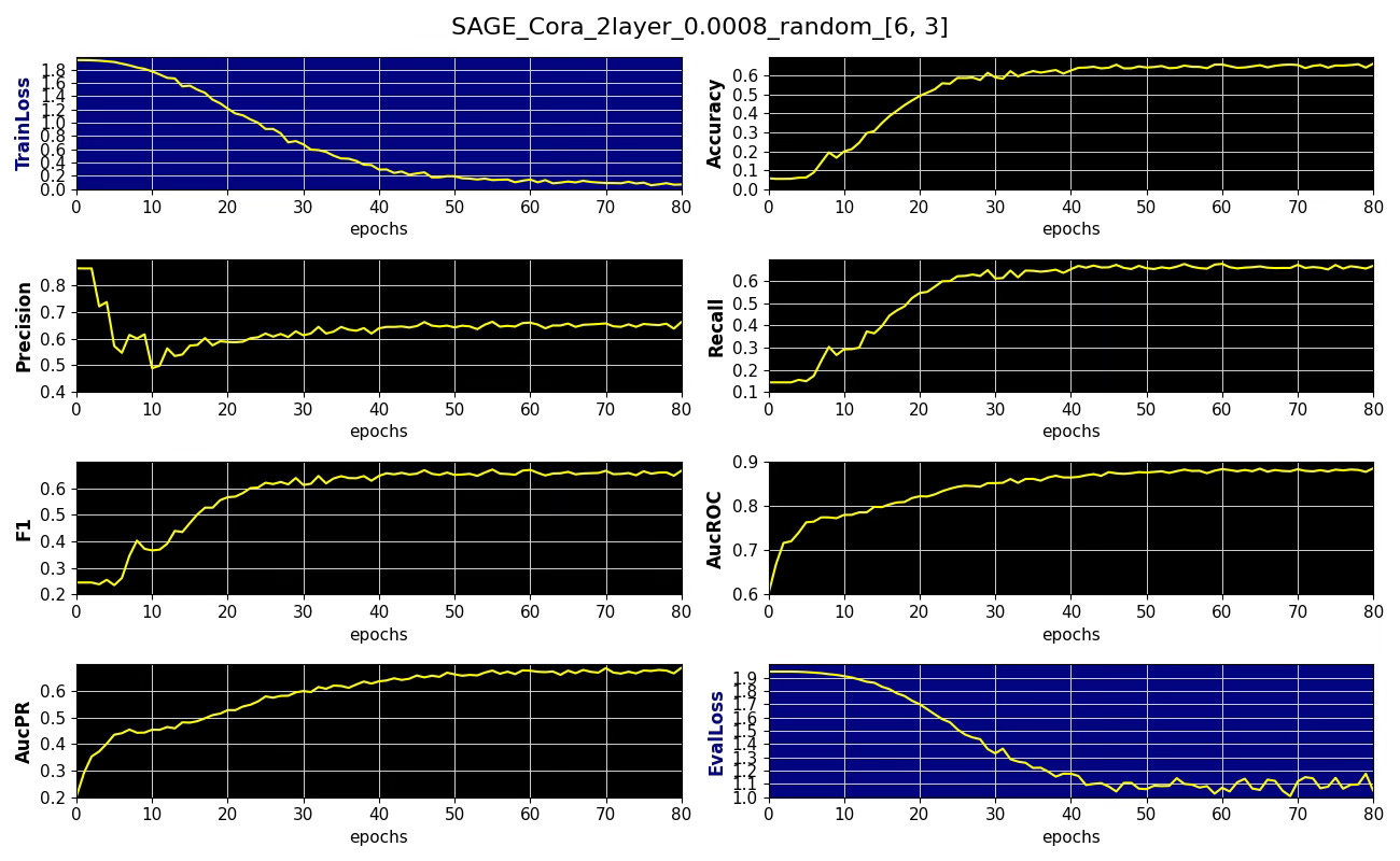
Fig. 3 Performance metrics, training and validation losses for node classification on Cora dataset with 6 x 3 node sampling aggregation, learning rate 0.0008

PubMed dataset configuration:

Sampling: {'id': 'NeighborLoader', 'num_neighbors': [12, 8],      
           'batch_size': 32, 'replace': True, 'num_workers': 4}
Number graphs: 1
Number nodes: 16000
Number features: 500
Number classes: 3
Is directed: False
Has loop: False
Training nodes: 50
Validation nodes: 393
Subgraph coverage: 0.811

Here is an example of performance metrics for 12 x 8 neighboring node sampling

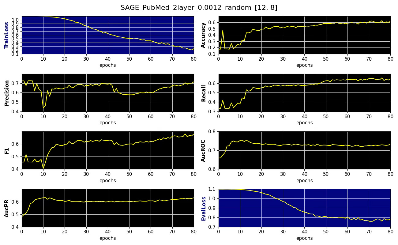
Fig. 4 Performance metrics, training and validation losses for node classification on PubMed dataset with 12 x 8 node sampling aggregation, learning rate 0.0012

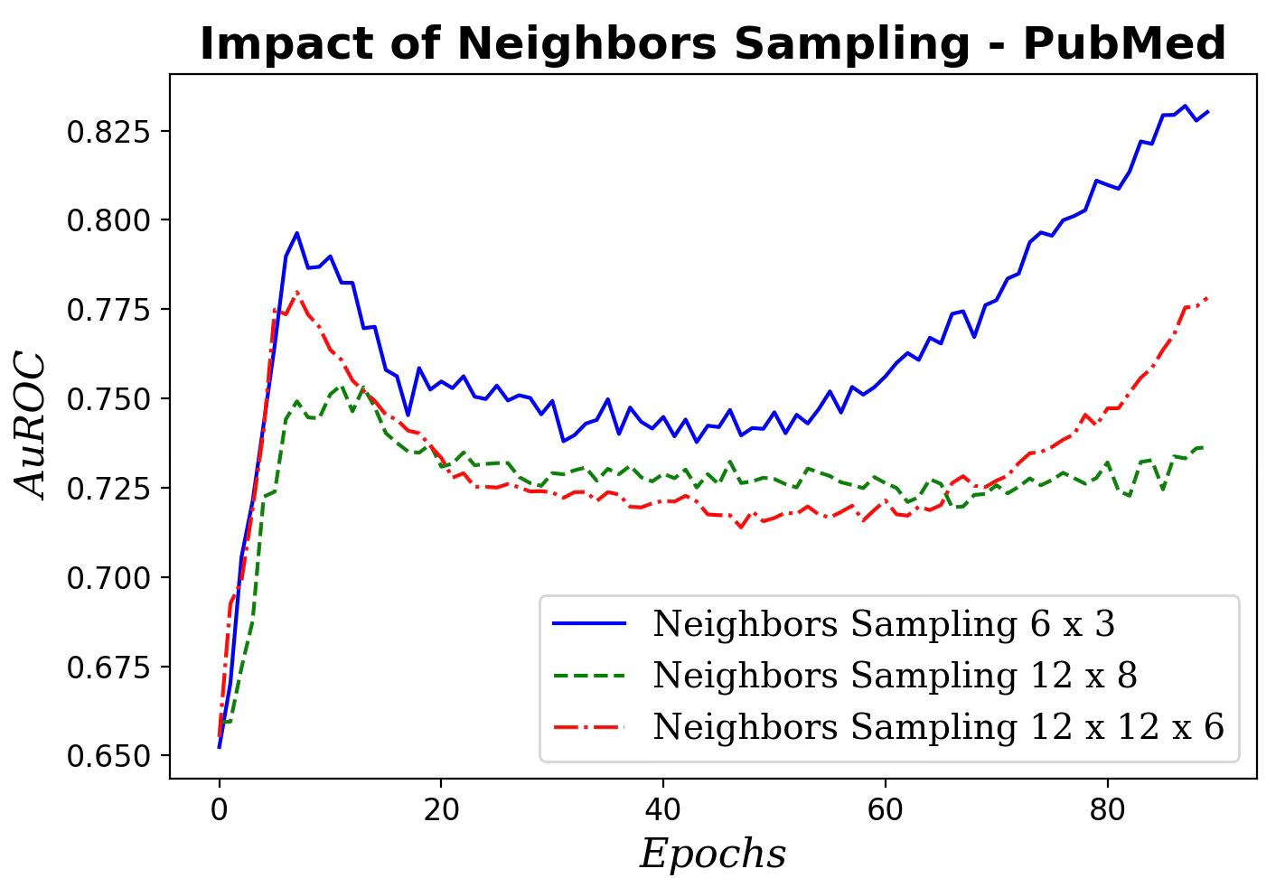
Fig. 5 Impact of neighboring nodes sampling for message aggregation on AuROC

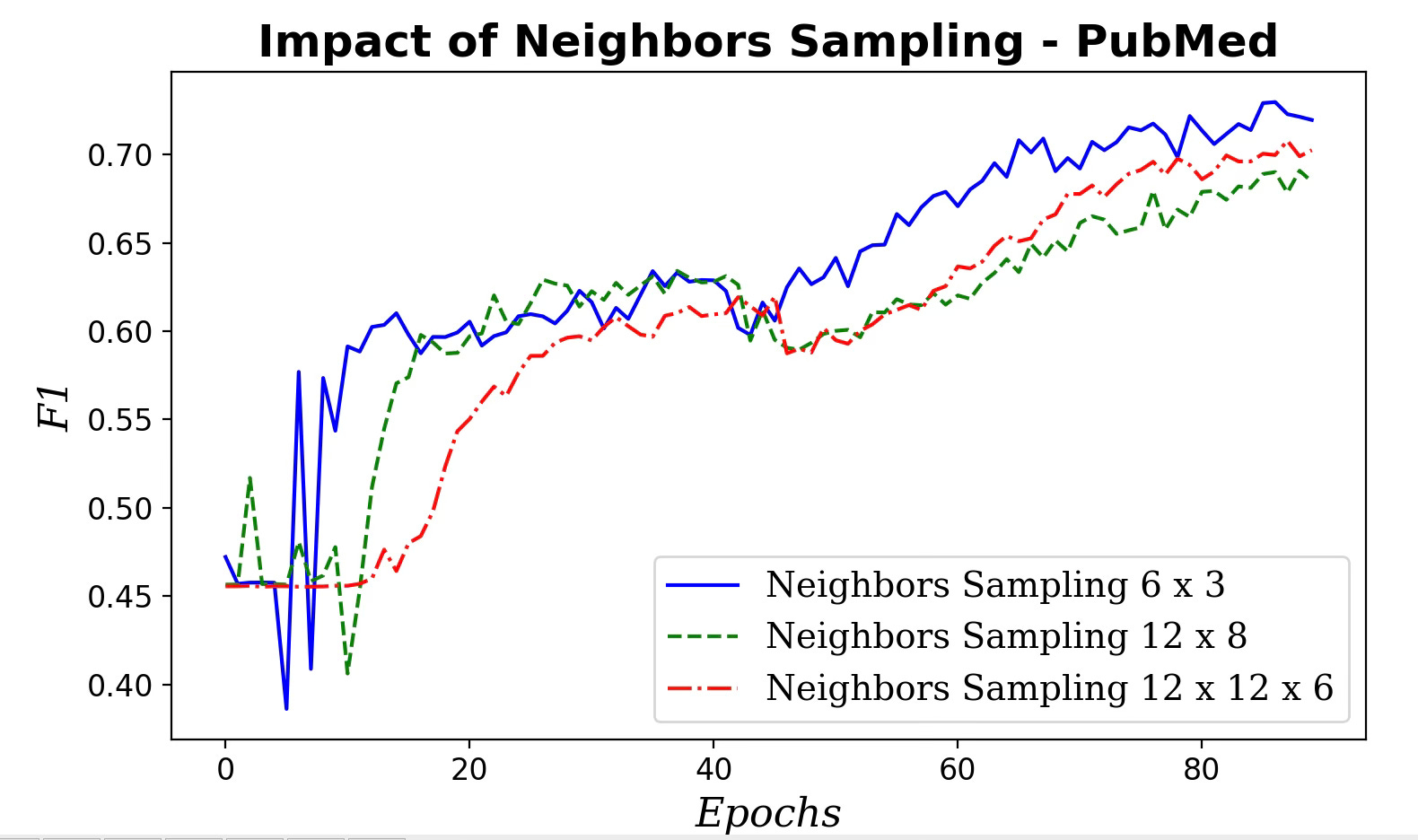
Fig. 6 Impact of neighboring nodes sampling for message aggregation on F1 metric

Clearly the performance of our GraphSAGE model decreases as the number of neighbors and hops used in aggregating message increases.

📌 Start with small neighbor sets for aggregation—often a single hop is best. Going beyond two hops can degrade performance.

Number of convolutional layers

In this scenario we evaluate the impact of number of SAGE convolutional modules (2 vs 3 SAGE layers).

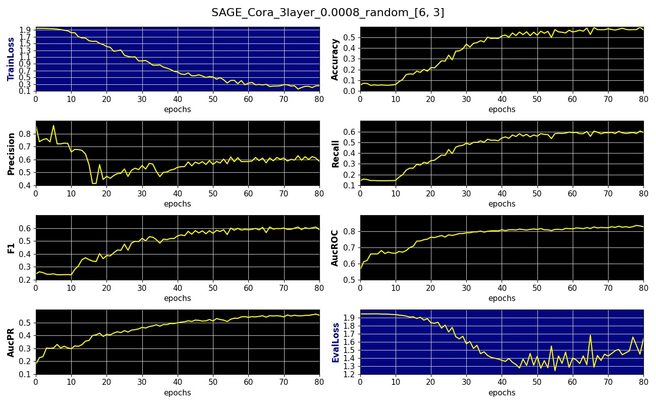
Fig. 7 Performance metrics, training and validation losses for node classification on Cora dataset with 6 x 3 node sampling aggregation, learning rate 0.0012 and 3 convolutional. layers

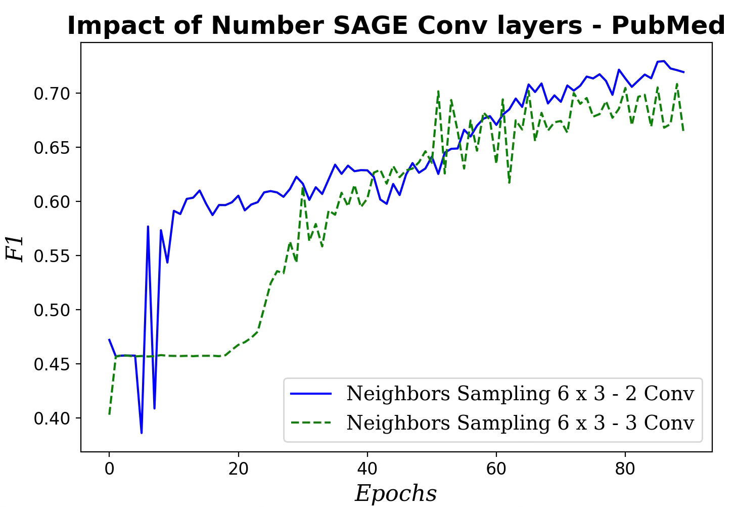
Fig. 8 Impact of number of SAGE convolutional layers on F1 metric

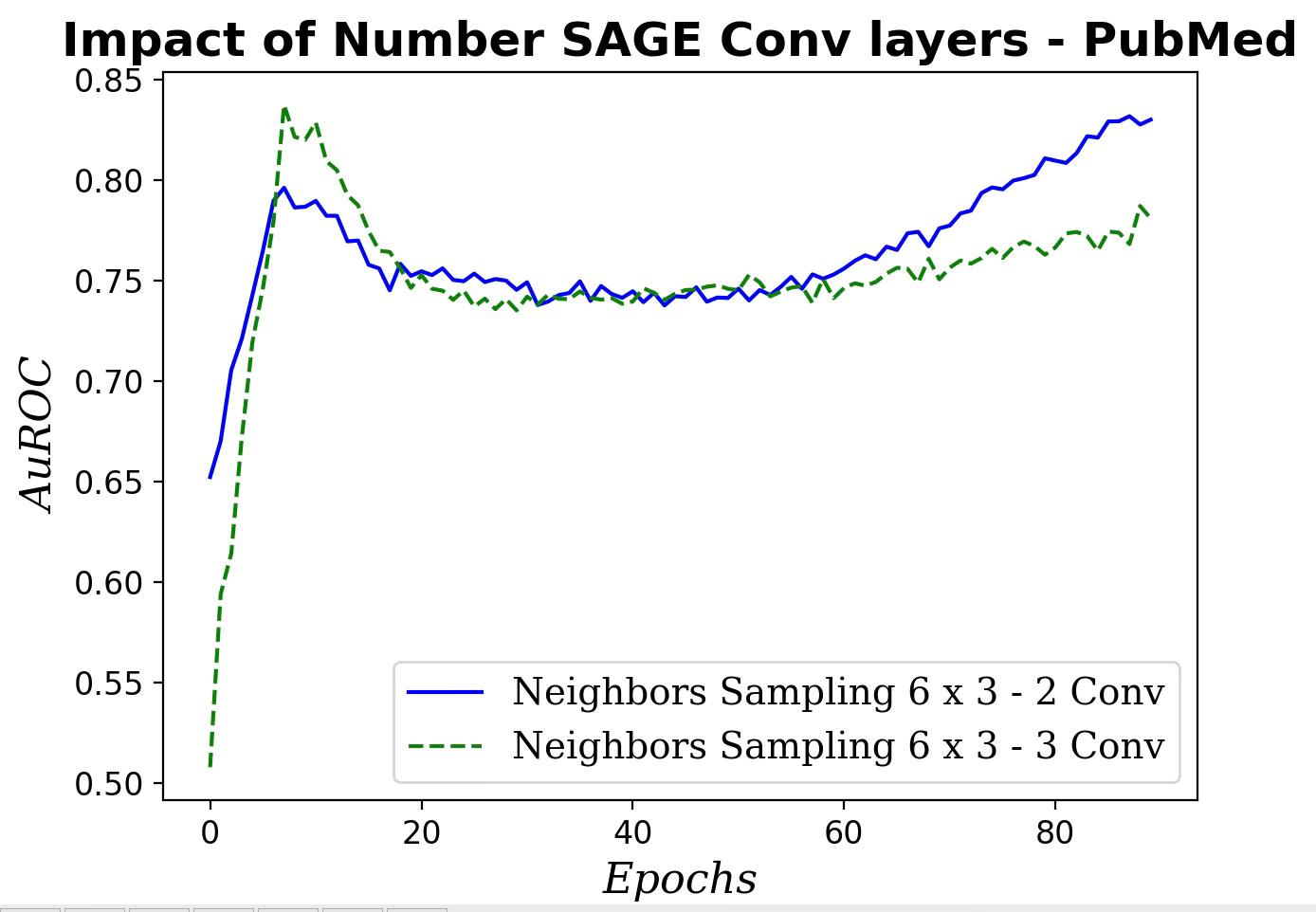
Fig. 9 Impact of number of SAGE convolutional layers on AuROC

Increasing the number of SAGE convolutional layers has a very limited impact on the performance of our GraphSAGE model.

Graph Sub-sampling & Latency

Lastly, we investigate the impact of sub-sampling the graph dataset on the performance metric and latency using the large graph dataset Flickr.

Sampling: {'id': 'NeighborLoader', 'num_neighbors': [20, 12], 
           'batch_size': 32, 'replace': True, 'num_workers': 4}
Number graphs: 1
Number nodes: 12000
Number features: 500
Number classes: 7
Is directed: False
Has loop: False
Training nodes: 6072
Validation nodes: 2962
Subgraph coverage: 0.134

Fig. 10 Performance metrics, training, validation losses for node classification on Flickr dataset with 20x12 nodes sampling aggregation, learning rate 0.0018 and 12K random subgraph

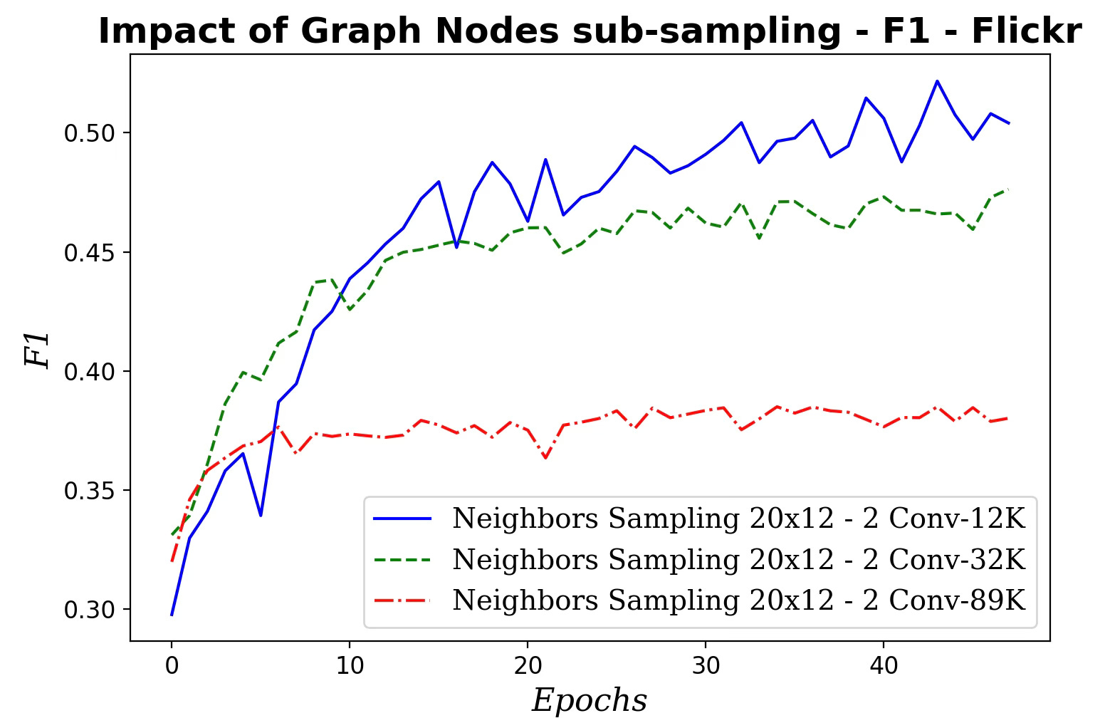
Fig. 11 Impact of the size of the sampled subgraph on F1 metric - Flickr dataset

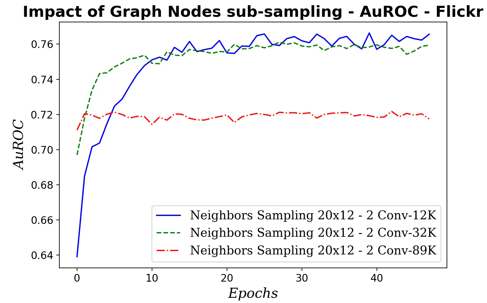
Fig. 12 Impact of the size of sampled subgraph on AuROC - Flickr dataset

Surprisingly, performance degrades as the subgraph grows, suggesting overfitting because the added nodes offer minimal additional variability. The likely causes of this results can be attributed to:

Sampling may distort edge-homophily, changing the fraction of same-label edges.
A significant percentage of nodes lie at the subgraph’s edge with truncated neighborhoods, downgrading the quality of aggregation.
Hubs may be over/under-represented affecting the neighborhood statistics.
Larger subgraphs with deeper/higher-hop aggregation blur features more than on the full graph.
Labels associated with the subgraph may have a different distribution that the entire graph
Sampling may alter degree, means or variances.

Being said, training a graph node classifier on a randomly sampled subgraph reduces computation load.

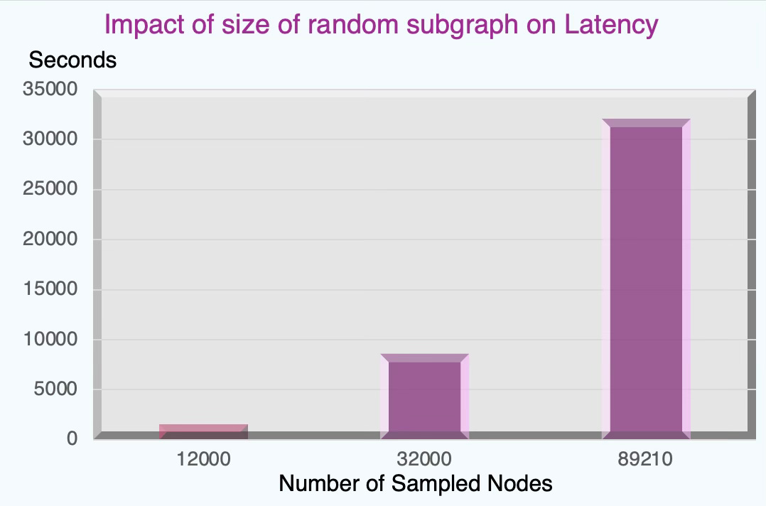
Fig. 13 Impact of the size of sampled subgraph on latency - Flickr dataset

🧠 Key Takeaways

✅ GraphSAGE is inductive: it doesn’t require processing the entire graph, making it often more efficient than full-graph (transductive) GNNs.

✅ Bigger neighborhoods can hurt: increasing hops or sampled neighbors may reduce performance (e.g., F1, AUROC).

✅ Deeper isn’t much better: adding more SAGE convolution layers has only a minor effect on this model’s performance.

✅ Subsampling is delicate: as the sampled subgraph grows, performance can drop due to more cross-class neighbors (low homophily) and distribution shift.

🛠️ Exercises

Q1: Does increasing the hop count in neighbor sampling improve node-classification performance?
Q2: What is the rationale for randomly sampling a subgraph from a large graph for node classification?
Q3: How does adding more GraphSAGE convolutional layers affect node-classification performance?
Q4: What challenges arise when extracting random subgraphs from large graphs, and how do they impact classifier performance?
Q5: Beyond layer depth and neighborhood sampling, which other model or training parameters most influence GraphSAGE performance?

Answers

Thanks for reading Hands-on Geometric Deep Learning! Feel free to share it.

Taming PyTorch Geometric for Graph Neural Networks Hands-on Geometric Deep Learning - 2025
Plug & Play Training for Graph Convolutional Networks Hands-on Geometric Deep Learning - 2025
GraphSAGE: Inductive Representation Learning on Large Graphs J. Leskovec, SNAP - Stanford University
Inductive Representation Learning on Large Graphs. W.L. Hamilton, R. Ying, and J. Leskovec 2017.
Reusable Neural Blocks in PyTorch & PyG Hands-on Geometric Deep Learning - 2025
Block by block: Rethinking Deep Learning Architecture Hands-on Geometric Deep Learning - 2025
Taming PyTorch Geometric for Graph Neural Networks: Graph Loaders Hands-on Geometric Deep Learning - 2025
Demystifying Graph Sampling & Walk Methods Hands-on Geometric Deep Learning - 2025

💬 News & Reviews

This section focuses on news and reviews of papers pertaining to geometric deep learning and its related disciplines.

Paper review: Flow Matching on Lie groups. F, Sherry, B. Smets CASA & EAISI, Dept. of Mathematics & Computer Science, Eindhoven University of Technology, the Netherlands

Flow matching has been extensively explored in Euclidean spaces using linear conditional vector fields. However, extending this concept to Riemannian manifolds poses challenges. A natural idea is to replace straight lines with geodesics, but this often becomes intractable on complex manifolds due to the difficulty of computing geodesics under arbitrary metrics.

To address this, the authors propose an alternative approach based on Lie group exponential maps, which is particularly effective for Special Orthogonal (SO(n)) and Special Euclidean (SE(n)) groups, leveraging efficient matrix operations.

Their method approximates the vector field induced by a Riemannian metric using a neural network. The conditional vector field is guided by an exponential curve—i.e., the exponential map applied to a Lie algebra element derived from a group element at time tt.

The model is evaluated on SO(3), SE(2), product groups, and homogeneous spaces, demonstrating strong alignment between the learned and target distributions—especially when the exponential curves are not overly complex.

Notes:

Source code and animations are available on GitHub.
The paper assumes readers are familiar with differential geometry, Lie groups, and Lie algebras.

Expertise Level

⭐ Beginner: Getting started - no knowledge of the topic
⭐⭐ Novice: Foundational concepts - basic familiarity with the topic
⭐⭐⭐ Intermediate: Hands-on understanding - Prior exposure, ready to dive into core methods
⭐⭐⭐⭐ Advanced: Applied expertise - Research oriented, theoretical and deep application
⭐⭐⭐⭐⭐ Expert: Research , thought-leader level - formal proofs and cutting-edge methods.